Basic DIY microphone design—Part 2: microphone front-end design

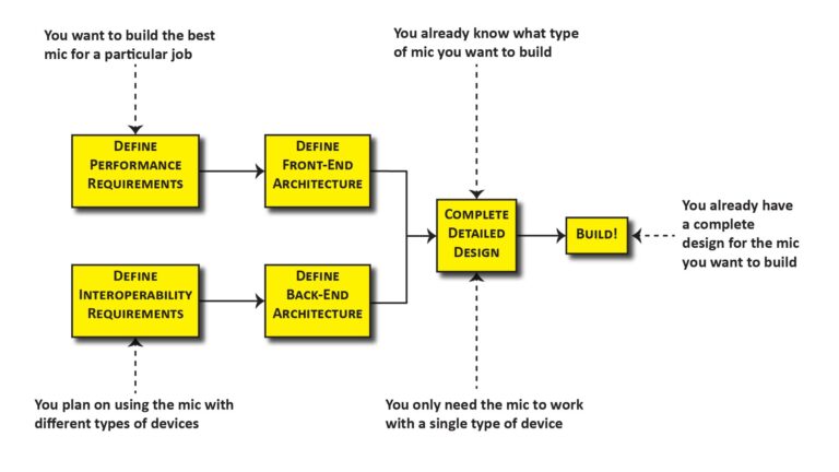
This post is about microphone front-end design: it shows how a microphone’s performance requirements drive key aspects of its design.

The microphone front-end

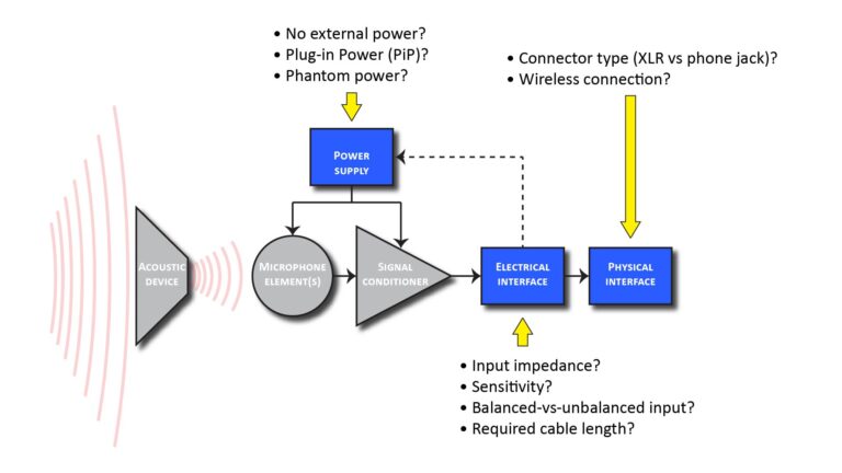
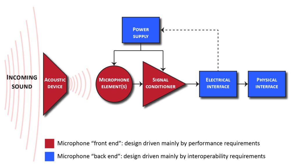
In Part 1 of this series (Basic DIY microphone design—Part 1: the microphone design process), I discussed the overall microphone design process and how a microphone can be decomposed into a front-end (that largely determines performance) and a back-end (that largely determines the types of devices the microphone can be used with). This post is about the microphone front-end, consisting of the items shown in red in the following block diagram:

How performance requirements drive microphone front-end design

My post on the 4 key microphone performance specs discusses the “big four” specs (polar response, Equivalent Input Noise, maximum SPL, and effective bandwidth), and describes the process for choosing them for a given usage scenario.

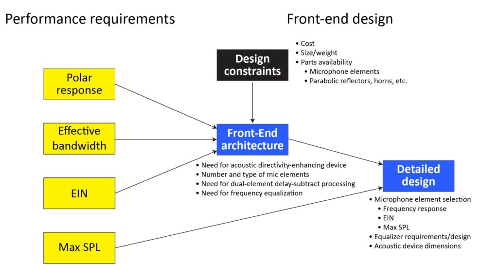
But along with those performance requirements—and as with the design of any type of device—there are also practical constraints like cost, size/weight, and the availability of the necessary parts. These two sets of considerations drive the microphone front-end design as shown in the following figure:

Defining the microphone front-end architecture

As with any electronic device, there are theoretically an infinite number of microphone architectures that could meet a particular set of performance specs.

However, there are far fewer practical microphone architectures. I’ve come across just six basic architectures that are worth considering for practical DIY microphones. From a design standpoint, these six architectures are distinguished by the type of microphone element(s) used (either pressure or pressure-gradient), whether an acoustic directivity-enhancing device (such as a parabolic reflector) is used, and whether there are more than one element in a differential array configuration (which requires delay-and-subtract signal processing).

We can begin the process of choosing the final front-end architecture from among these six choices on the basis of the polar response we need.

Required polar pattern drives microphone front-end architecture

From a microphone design standpoint, it’s useful to group polar patterns into three regimes: the isotropic polar pattern, the standard directional patterns (bidirectional, cardioid, supercardioid, and hypercardioid), and various high-directivity polar patterns (such as those provided by a shotgun microphone). This section of my post on microphone specs discusses the characteristics of these patterns and when they’re useful, while the following chart shows the microphone front-end architectures (the black boxes) needed to provide each of these three polar pattern regimes:

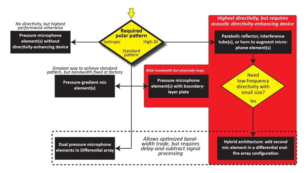
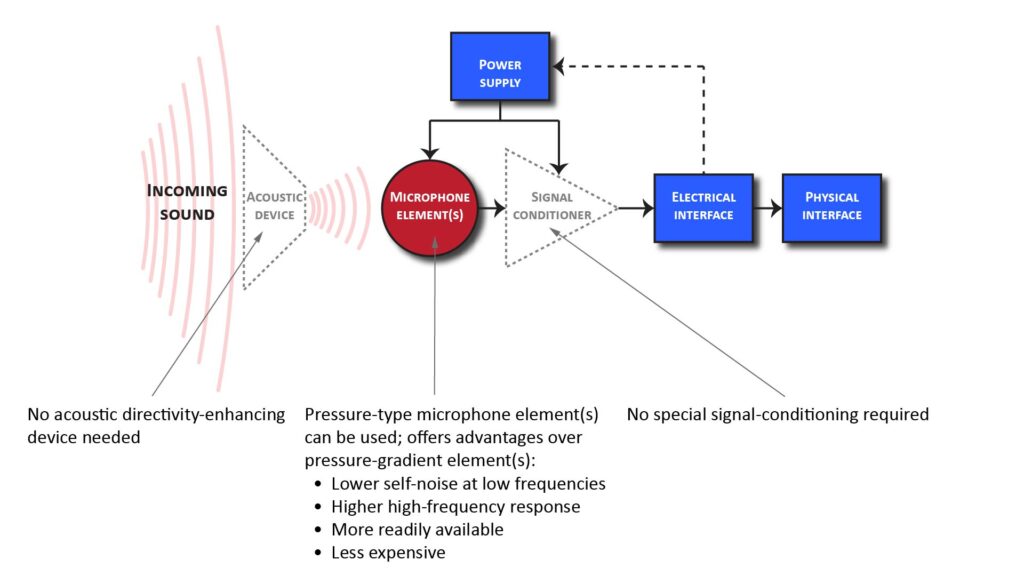
Microphone front-end architecture for an isotropic polar pattern

If no directivity is needed, there’s just one basic front-end architecture to choose from, as shown on the top left of Figure 3—and it’s the simplest (and in many ways also the best) front-end-architecture.

An isotropic pattern doesn’t require an acoustic directivity-enhancing device (like a parabolic reflector), special signal processing, or a pressure-gradient microphone element:

When would we want an isotropic pattern?

Some microphone applications either don’t benefit from directivity or else actually require an isotropic response. For example, if there’s relatively little ambient noise, there’s no need to limit the mic’s polar response to just the direction of the intended sound source. And if there are multiple sound sources, or if a specific orientation of the mic with respect to the sound source(s) can’t be guaranteed (such as with a lavalier mic), then directivity could actually degrade performance.

Further, a microphone with an isotropic response is capable of providing the best possible performance in all aspects other than directivity. Thus, the isotropic configuration makes for an excellent and easy-to-build general-purpose microphone.

Microphone front-end architectures for the standard polar patterns

As explained in the polar response section of my post on microphone specs, there are four standard directional polar patterns: the bidirectional, cardioid, supercardioid, and hypercardioid patterns. Such patterns can be achieved with three different front-end architectures discussed below.

Using an actual pressure-gradient microphone element

The simplest way to implement a standard polar pattern is with a pressure-gradient microphone element, as shown in Figure 5 below:

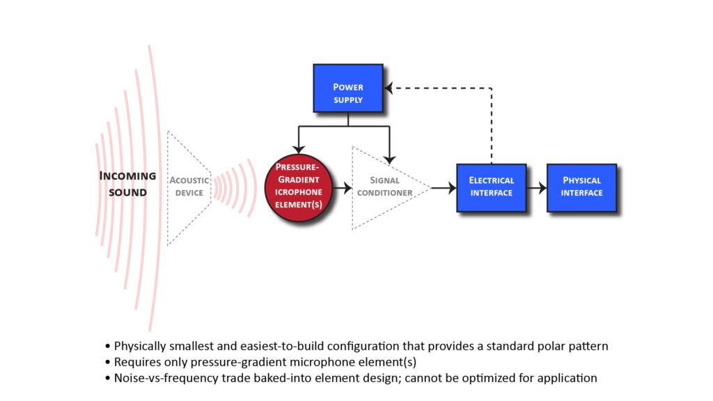
Such an element produces an output that’s a function of the difference in acoustic pressures at two points on either side of a single diaphragm; varying the distance and attenuation between each point and the diaphragm allows any of the standard polar patterns to be realized.

Pressure-gradient elements with bidirectional (figure-eight), unidirectional (cardioid, supercardioid, and hypercardioid) patterns are available, although the variety of some of these types is limited.

Implementing a virtual pressure-gradient microphone via a differential array

Instead of using an actual pressure-gradient microphone element, a virtual pressure-gradient microphone can be implemented by using two pressure elements followed by a delay-and-subtract processor, as shown in Figure 6 below:

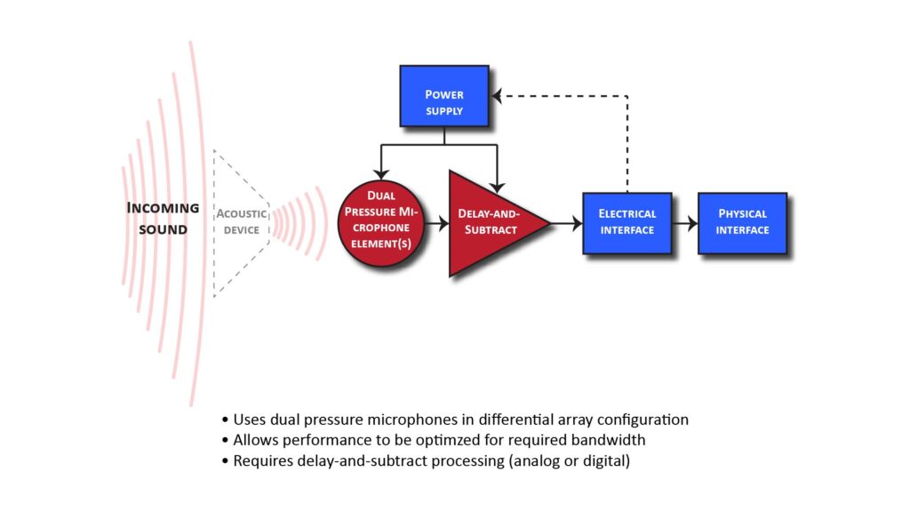
This is sometimes called a dual-element (or first-order) differential array (by the way, array microphones are described in detail in my post on how array microphones work).

Such a virtual pressure-gradient microphone works in exactly the same way as an actual pressure-gradient element: the delay-and-subtract processing electronically emulates what happens acoustically across the diaphragm of a pressure-gradient element, and any of the standard patterns can be achieved by varying the delay and gain.

The delay-and-subtract processing can be implemented in at least three ways:

• In real-time, using analog circuitry built-into the microphone itself. This offers high performance and compact packaging, but the circuitry can be somewhat complex for someone who isn’t comfortable with electronics (especially if the polar pattern must be electronically adjustable).
• In real-time, using a DIY Digital-Signal Processor (DSP) box (based on an off-the shelf DSP board) connected between two microphone systems and the downstream audio device. This is physically somewhat cumbersome (requiring two microphone mounts and associated cabling) and typically has a higher noise floor than the analog approach, but is much easier to implement and allows the performance parameters to be reprogrammed at any time.
• In non-real-time using a Digital Audio Workstation (DAW) to process separate recorded tracks from two microphones. This is the most flexible approach and requires no hardware fabrication, but sacrifices real-time operation and also requires two microphone mounts and associated cabling.

Using a pressure microphone element with a boundary-layer surface

Another way to implement a cardioid-like pattern (but not any of the other standard patterns) is a boundary-layer microphone, as shown in Figure 7 below:

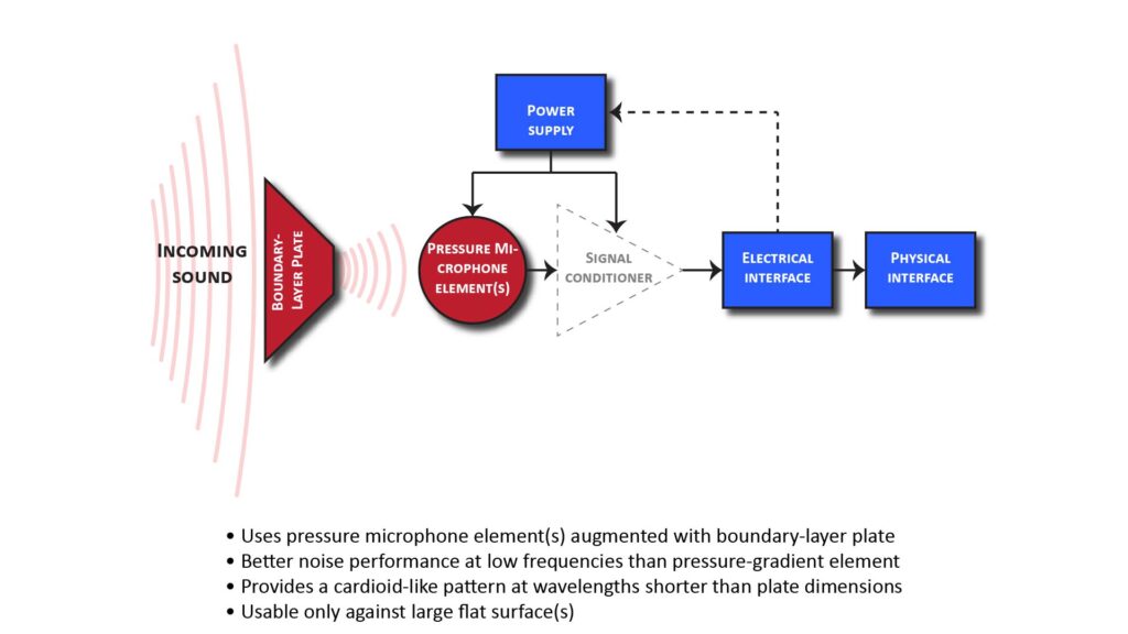
A boundary-layer microphone consists of one ore more pressure-type (isotropic) elements mounted flush on a large flat “boundary-layer” surface. As mentioned above, this provides a “cardioid-like” pattern because it’s sensitive only to sounds in the hemisphere in front of the flat surface, so—like a cardioid pattern—it provides a Directivity Index of 3 dB. Unlike a cardidoid pattern, it also provides a sensitivity gain of 6 dB (which effectively increases the microphone element’s signal-to-noise ratio by 6 dB). This can make a boundary microphone useful when very low self-noise is needed, such as for capturing sound in a quiet studio.

However, unlike a real or virtual pressure-gradient microphone, a boundary microphone’s directivity and gain are maintained only down to wavelengths comparable to the size of the flat surface. So, because a large boundary-layer surface is required to maintain directivity down to bass frequencies, the boundary-layer approach is advantageous only for microphones mounted on a wall, floor, or conference-room table.

When would we want a standard polar pattern?

Before we discuss the advantages and disadvantages of each of the architectures of Figures 5 – 7, let’s review why we might want a standard polar pattern in the first place. A standard polar pattern can offer three key benefits:

• Direction-specific noise suppression. A microphone with even modest directivity can have very deep off-axis nulls in its polar pattern, and pointing one of those nulls toward a noise source can greatly reduce the effects of that noise. In fact, a bidirectional or cardioid microphone can often rival the performance of a high-directivity microphone (like a parabolic type) in the presence of anisotropic noise.
• Spatial sampling for multi-channel recording formats. The enhanced realism provided by multi-channel recording formats like stereo, Ambisonics, and surround-sound is enabled by microphones with standard directional patterns (typically bidirectional or cardioid types).
• Modest range extension in the presence of isotropic ambient noise. If there’s significant isotropic ambient noise (such as in a room with a lot of reverberation), a mic with an isotropic polar pattern may have to be placed very close to the source (perhaps just a few inches) to capture sound with acceptable quality, whereas a microphone with a standard pattern can allow the source-to-mic distance to be increased (by as much as a factor of two) while maintaining the same signal to ambient noise ratio.

Comparing the architectures for achieving a standard pattern

The fact that a boundary microphone needs to be used in proximity to one or more large, flat surfaces limits its potential applications, and also means that it can’t be used for direction-specific noise suppression or capturing sound for multi-image recording formats. However, when it can be used, a boundary microphone can out-perform real or virtual pressure-gradient microphones; we’ll see why shortly.

One unique advantage of real and virtual pressure-gradient microphones over boundary-layer microphones (and over the high-directivity microphone configurations we’ll discuss later) is that they maintain their directivity at low frequencies. That’s a huge advantage, because ambient noise usually has a lot of power at low frequencies.

However, a pressure-gradient microphone also has two unique disadvantages:

• Both the directivity and the on-axis frequency response degrade above a certain frequency (due to aliasing in the polar pattern and frequency domain).
• There is an inherent 6-dB-per-octave roll-off with decreasing frequency over the entire usable bandwidth.

In fact, the design of a pressure-gradient microphone represents a trade between minimum and maximum usable frequencies: the higher the maximum usable frequency, the poorer the response at low frequencies. For example, a pressure-gradient microphone designed for an alias-free on-axis response up to 20 kHz will have an inherent roll-off of 33 dB at 300 Hz, whereas one that’s designed to operate up to 10 kHz will have an inherent roll-off of 27 dB at 300 Hz.

Those huge low-frequency roll-offs have to be dealt with somehow. In off-the-shelf pressure-gradient microphones, this is done by adjusting the diaphragm mass to provide a 6-dB-per-octave high-frequency roll-off that exactly compensates the inherent low-frequency roll-off; the result is a virtually flat frequency response. The same thing can be done electronically in a differential array microphone: we can either boost the low frequencies or cut the high frequencies by 6 dB per octave to achieve a near-flat response.

However, there’s a catch: whether we boost the lows or cut the highs, the inherent low-frequency roll-off is still there, and it degrades the signal-to-noise ratio at low frequencies. It’s like having a microphone with a much higher self-noise at low frequencies. And if the effective self-noise is high enough, it can dominate the overall noise at the microphone output—negating the benefit of any ambient noise suppression provided by the modest 6 dB of directivity.

In fact, this effect can cause the overall performance of a pressure-gradient microphone to actually be worse than that of an isotropic microphone in the presence of a modest amount of ambient noise. That doesn’t usually happen, but it’s something to be aware of, and I’ll discuss it more later in this post.

This brings up one of the advantages of a virtual pressure-gradient microphone over an an actual pressure-gradient microphone element. In an actual pressure-gradient microphone, the aforementioned trade between minimum and maximum usable frequencies is baked-into the design of the microphone element. And virtually all off-the-shelf pressure-gradient microphone elements are designed to have a maximum usable frequency of at least several kHz, which results in a huge inherent roll-off at bass frequencies (and therefore, poor noise performance at those bass frequencies).

But with the array approach, we can optimize the bandwidth to suit the application. For example, we can build a microphone that trades away some bandwidth at the upper end for improved noise performance at the lower end. I’ll discuss why we might want to do that a bit later in this post.

The following table summarizes the advantages and disadvantages of the three architectures of Figures 5 – 7:

	Actual pressure-gradient element(s)	Virtual pressure-gradient microphone (differential array)	Boundary-layer microphone
Achievable polar pattern	Bidirectional, cardioid, supercardioid, hypercardioid (although choice may be limited for certain element types)	Any “first order” pattern, including all standard patterns	Pseudo-cardioid (same directivity as cardioid, but also provides sensitivity gain)
Applications	Anisotropic noise suppression, spatial sampling, modest range extension	Anisotropic noise suppression, spatial sampling, modest range extension	Modest range extension, low-noise studio recording
Physical constraints	None	None	Must be used in proximity to one or more large flat surfaces
Required signal processing	None	Delay-and-subtract	None
Bandwidth-noise trade	Determined by microphone element design	Determined by element spacing and processing parameters	Not an issue

Microphone front-end architectures for high directivity polar patterns

As previously shown in Figure 3, there are two microphone front-end architectures that can provide significantly greater directivity than the standard polar patterns:

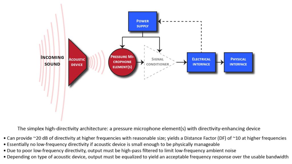
• We can use an acoustic directivity-enhancing device (such as a parabolic reflector or an interference tube) with a pressure-type microphone element. I’ll call this the simplex architecture as shown in the block diagram of Figure 8 below. By the way, I discuss the most practical directivity-enhancing devices in detail in my post on long-range directional microphones.
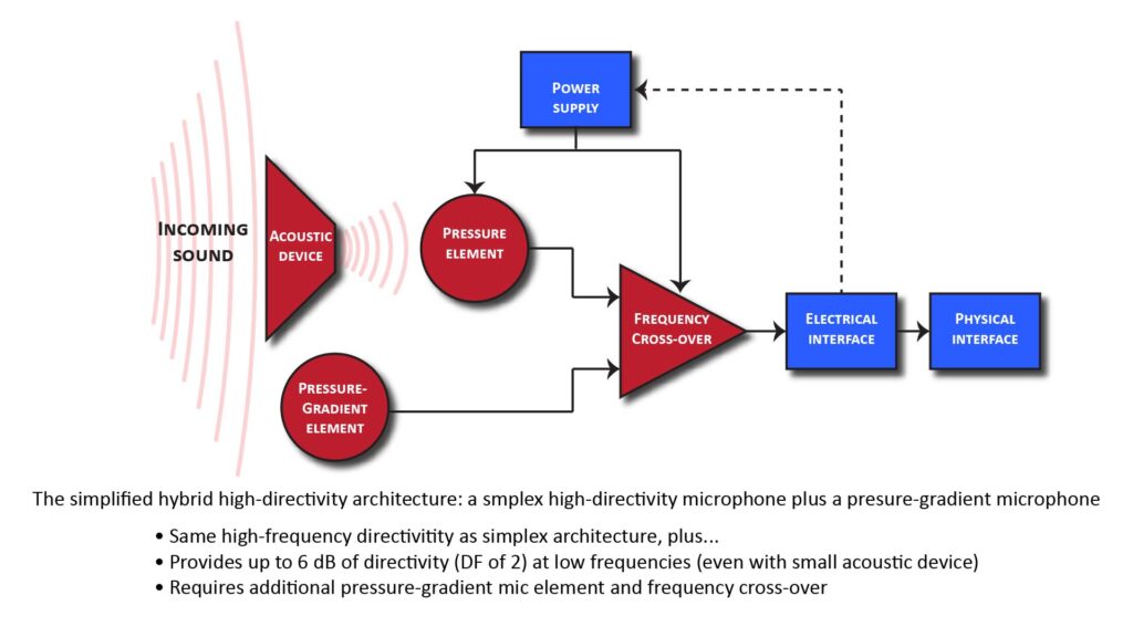
• Acoustic directivity-enhancing devices are effective only at wavelengths comparable to, and shorter than, their physical dimensions. But what if we need directivity at low frequencies, but can’t use a physically large device? The solution is to combine the output of a simplex high-directivity microphone with that of a second microphone element. This can be done in the time-domain (which I’ll call the hybrid architecture as shown in Figure 9) or in the frequency domain (which I’ll call the simplified hybrid architecture, shown in Figure 10).

Before we discus these three approaches, let’s review why we might want a high-directivity polar pattern.

Why would we want a high-directivity polar pattern?

The classic use-case for a high-directivity polar pattern is for picking-up sounds at long ranges, as discussed in detail in my post on long-range directional microphones. High directivity is essential for long-range pick-up because the SPL of the desired sound is typically far below the ambient noise level when it reaches the microphone; the high directivity suppresses the ambient noise, allowing the desired sound to emerge above the noise floor.

The key performance metric for long-range pick-up with a directional microphone is the Distance Factor (DF), which is the factor by which the pick-up range is increased relative to that of an isotropic microphone (for reference, a hypercardioid pattern—which has the highest directivity of all the standard patterns—has a DF of 2).

There are two range regimes in which the greater DF of a high-directivity polar pattern can be useful:

• Ranges just beyond the capabilities of a standard hypercardioid pattern. The classic use-case is for moving a microphone out of a camera’s field-of-view in video production; this can require a range of several feet (or a DF of something like 4). Such an application usually also requires high fidelity.
• Ranges far greater than possible with a standard hypercardioid pattern. Classic use-cases are for surveillance and sports applications; you can never have enough DF in such applications, but a DF of at least 10 is usually needed. Fortunately, such applications can usually tolerate relatively poor fidelity.

Comparing the simplex and hybrid architectures

Aside from the need for a potentially large acoustic directivity-enhancing device, the simplex approach of Figure 8 has one major limitation: the directivity provided by an acoustic directivity-enhancing device depends on its size in wavelengths. Specifically, in order to provide significant directivity, at least one physical dimension (depending on the type of device) must at least a wavelength long.

The practical implication is that while a reasonably-sized directivity-enhancing device can provide a DF of, say, 10 or more at high frequencies, it will provide a DF of only 1 at low frequencies.

This also means that a reasonably-sized device cannot suppress low-frequency ambient noise, so the only way to control low-frequency noise is to high-pass filter the microphone’s output—which unfortunately also eliminates the “good” low frequencies in the desired sound. Fortunately, as previously mentioned, applications that require high DFs can usually accept the compromise in fidelity that comes from high-pass filtering.

Advantages of the hybrid architecture

In view of the above, it’s obvious that the 6 dB of low-frequency directivity (which corresponds to a DF of 2) provided by the hybrid approaches of Figures 9 or 10 would be advantageous in any application that calls for high directivity. However, whether it’s advantageous enough to be worth the added complexity is a different question.

The less the high-frequency directivity provided by the acoustic device, the relatively more valuable would be the 6 dB of low-frequency directivity provided by the delay-and-subtract signal processing. For example, if the acoustic device provides a high frequency directivity of just 12 dB (corresponding to a DF of 4), then the 6 dB of added low-frequency directivity can make a substantial difference.

In fact, all modern shotgun microphones (which have high-frequency directivities of the order of 10 dB) use a hybrid approach: they rely on an acoustic directivity-enhancing device (specifically an interference tube) at higher frequencies, but act like a pressure-gradient microphone at lower frequencies. BTW, I discuss shotgun microphones in detail in A deep look at how shotgun microphones really work.

On the other hand, if the acoustic device provides a high-frequency directivity of as much as, say, 20 dB (corresponding to a DF of 10), then the 6 dB of low-frequency directivity provided by the delay-and-subtract processing might not be enough to justify the added complexity. In fact, as far as I’m aware, there aren’t any large commercial parabolic microphones (which have high frequency directivities of 20 – 30 dB) that use a hybrid approach.

In short, the hybrid approach makes sense whenever only modest ranges (and hence DFs) are needed, but might not be cost-effective when long ranges (and hence high DFs) are needed, such as in applications for large parabolic mics.

Where the hybrid architecture makes sense

A good candidate for the hybrid architecture is a relatively small parabolic microphone, such as the Klover MiK 09 by Klover Products, Inc. This device is intended as a higher-performance alternative to conventional shotgun microphones, but still has a peak directivity low enough that overall performance can be substantially increased using a hybrid approach. If you’re interested, I provide projections of the increased pick-up range possible with the hybrid approach in my review of the Mik 09 (“The Klover MiK 09: can a small parabolic microphone outperform a shotgun microphone?“).

Implementing the hybrid architecture

There are many ways to implement the hybrid architecture, but Figures 9 and 10 show two of the most practical approaches.

In Figure 9, the outputs of two separate microphones (in this case two pressure elements) are combined using delay-and-subtract processing. On the other hand, in Figure 10, the outputs of two separate microphones (one pressure element and one pressure-gradient element) are combined using high-pass and low-pass filters.

Depending on the equipment you have on-hand, you might not need any additional hardware to implement either of these hybrid approaches.

For example, many prosumer-grade multitrack field recorders (such as the Zoom F6) have built-in time-alignment and channel-inversion capabilities to implement the delay-and-subtract processing of Figure 9. Similarly, the equalizer functionality built-into just about all Digital Audio Workstation (DAW) applications can implement the required frequency cross-over processing of Figure 10.

Stay tuned for posts on exactly how to do this.

Finalizing the microphone element configuration

Once the basic front-end-architecture is determined on the basis of the required polar response, the next step is to finalize the microphone element configuration. This involves making two decisions:

• We need to finalize the microphone element specifications (or, in more practical terms, choose the off-the-shelf microphone element that most closely meets our requirements). By the way, I have a post in the works on the best microphone elements for various DIY microphone application.
• We need to decide if a single microphone element will suffice, or if we need to use multiple microphone elements in an additive array configuration in order to to meet the microphone system’s Effective Input Noise (EIN) requirement.

The process is depicted in Figure 11:

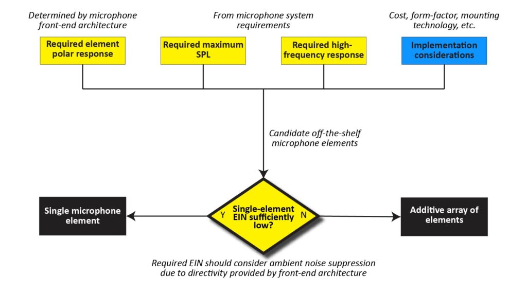
Finalizing the microphone element polar response

The required microphone element polar response is a fall-out from the basic microphone front-end architecture: per Figure 3, it will typically be an isotropic response (via a pressure microphone element) if we’re using an acoustic directivity-enhancing device or a dual-element differential array configuration, or else it will be one of the standard polar patterns (via a pressure-gradient microphone element).

Finalizing the high-frequency response and max SPL specifications

Regardless of a microphone system’s front-end architecture, its high-frequency response and maximum Sound-Pressure Level (SPL) will be limited by the microphone element: if we need bandwidth that extends to 20 kHz, the element’s response must extend to 20 kHz, and if need distortion-free capture of 120 dB SPL, the element’s max SPL must be 120 dB SPL.

Therefore, the required element HF response and max SPL flow down directly from the microphone system requirements, as discussed in my post on the 4 key microphone specs.

Addressing implementation considerations

At this point we’ve identified the polar response, HF response, and max SPL we need for our microphone element(s). However, there are probably hundreds, if not thousands, of readily available microphone elements that could meet any given set of such requirements.

Therefore, this is the appropriate point in the design process to begin addressing implementation considerations other than performance to help narrow-down the element selection. Such considerations include:

• Cost
• Form factor
• Mounting technology

Note that I’m not including characteristics like sensitivity, output impedance, or bias/power requirements at this point because, while they do drive aspects of the microphone back-end design, they don’t have a first-order effect on the front-end design or system performance.

On the other hand, a microphone element’s cost, form factor, or mounting technology can be deal-breakers for a particular DIY microphone project. However, such considerations are in the realm of detailed design and are beyond the scope of this post (I’ll link to upcoming post on the subject here).

For now, the main point is that implementation considerations—in addition to polar response, HF response, and max SPL—will generally narrow-down the number of viable microphone elements to a manageable number.

Addressing the system Equivalent Input Noise (EIN) requirement

The final step in finalizing the microphone element configuration is to determine if just a single element will suffice, or if multiple elements in an additive array configuration are needed. This decision is based on the microphone system’s EIN requirement versus the EIN specs of candidate elements, less any ambient noise-suppression due to the directivity provided by the microphone front-end architecture:

• As discussed in the EIN section of my post on microphone specs, the microphone’s EIN should be comfortably below the lowest expected ambient noise level; I use a margin of 6 dB. So, if we expect to use the mic in a studio with an ambient noise level of 25 dB SPL, we want the effective microphone EIN to be no greater than 19 dB SPL.
• However, if the ambient noise is expected to be isotropic and we’re using a front-end architecture that provides a cardioid pattern (which has a directivity index of 4.8 dB), the ambient noise will be reduced by 4.8 dB. That’s a good thing, but if we still want the microphone EIN to be 6 dB lower than the ambient noise level, we need an EIN no greater than 14.2 dB.

If we can find a microphone element that meets all the other performance and implementation requirements and has a suitably low EIN, then our microphone front-end design is complete.

However, we might not be able to find an otherwise satisfactory element with a suitably low EIN. This might be the case, for example, if we’re building a high-performance studio microphone but want to avoid using an expensive externally-polarized condenser element that requires Phantom Power.

In that case, we could use an additive array configuration which consists of multiple microphone elements whose outputs are summed together. If each element has the same Signal-to-Noise Ratio (SNR), then the SNR at the output of the summing amplifier will be 10log(N) dB greater than the SNR of the individual elements (where N is the number of microphone elements). This increased SNR effectively reduces the EIN by the same amount (all this and more is discussed in detail on my post on how array microphones work).

So, for example, an additive array using ten microphone elements with an SNR of 70 dB each will have an overall SNR of 80 dB, which corresponds to an impressively low EIN of just 14 dB SPL.

There are at least two potential circumstances when an array configuration might make sense:

• When extremely low EINs are desired using Electret-Condenser Microphone (ECM) or MEMS (Micro-Electro-Mechanical Systems) elements. An EIN of less than 5 dB SPL can easily be achieved this way with relatively inexpensive elements.
• When a respectable EIN is needed with pressure-gradient elements. Pressure-gradient elements have higher EINs than pressure elements and are therefore more likely to benefit from an array configuration.

However, there is one performance caveat with an additive array: the microphones must be small and closely-spaced to avoid “beaming” (excessive directionality) at high frequencies. Fortunately, the microphone elements mostly likely to benefit from an array configuration (ECM and MEMS elements) are also likely to be physically small.

Wrap-up

As we’ve seen, a microphone’s front-end architecture specifies the type and number of microphone elements, the type of acoustic directivity-enhancing device (if any), and the type of special signal-conditioner (such as a delay-and-subtract signal processor).

The required front-end architecture flows directly from the microphone’s performance requirements, and defining it is the first step in the overall microphone design process (as described in Part 1 of this series).

Next up: Part 3 of this series, in which I discuss how a microphone’s back-end architecture is determined by its interoperability requirements.