Predicting microphone performance—Part 3: microphone range prediction

Unfortunately, the internet doesn’t provide detailed info on predicting microphone range in any one place…until now. This post describes methods to predict a microphone’s pick-up range as a function of its key performance attributes and required signal quality.

Prerequisites

This is Part 3 of a 3-Part series:

• In Predicting microphone performance—Part 1: what is microphone SINR?, I introduced the concept of the Signal-to-Interference-plus-Noise Ratio (SINR) as applied to microphones.
• In Predicting microphone performance—Part 2: using the SINR, I discussed each of the SINR variables, and show various ways in which the SINR can be used to quantify the quality of a microphone’s output signal.

This concluding post is about one of the most important applications for the SINR: estimating microphone range (which is the distance at which a particular microphone can pick-up sound of the required quality).

Why is this post necessary?

As you might know if you’re familiar with this site, I have an interest in long-range microphones like shotgun and parabolic types. Before I built my first such microphone, I looked online for information on predicting microphone range, or at least some credible range estimates for various types of long-range microphone.

Unfortunately, all of the range estimates I found online were anecdotal and poorly-documented, or else were just marketing claims from manufacturers or distributors. And I couldn’t find any coherent method of predicting microphone range that met my standards as an engineer.

Here are just a few of the specific range-related questions I had—and couldn’t find the answers to—when I embarked on my first long-range microphone project:

• One advantage of a parabolic microphone over a shotgun microphone is that the former provides gain as well as directivity, while the latter provides only directivity. But what impact does gain have on the usable microphone range?
• When building a long-range microphone, is there any range benefit to using a microphone element with low self-noise (aka Equivalent Input Noise), or is the range limited purely by ambient noise?
• By how much does the pick-up range of a long-range microphone decrease if it must capture high-quality voice (such as for video production) rather than just intelligible voice (such as for sports or surveillance applications)?
• Conversely, suppose we want to use a long-range microphone to detect the presence of voice (such as in a search-and-rescue application), rather than to pick-up intelligible voice; what’s the increase in range we can expect because we don’t care about intelligibility?

This series of posts on the Signal-to-Interference-plus-Noise Ratio (SINR) provides the answers. Part 1 and Part 2 laid the SINR groundwork; this final part is range-prediction methods using the SINR that can answer some of the questions mentioned above.

The fundamental assumption in predicting a microphone’s pick-up range: free-field propagation

Any reasonably practical prediction of microphone range depends on one crucial assumption: that the sound we want to pick-up is propagating under free-field conditions. Free-field propagation means that the sound’s wavefront is free to expand spherically as it travels away from the source.

With free-field propagation, the sound pressure falls-off with the square of the range (which is known as the inverse-square law), and the math needed to predict pick-up range is straightforward. Otherwise, the math gets extremely complicated.

Unfortunately, perfect free-field propagation almost never occurs in microphone applications, because there is usually at least one nearby surface (such as the ground) that prevents true spherical expansion.

However, propagation generally approximates free-field behavior, especially at the frequencies most important for voice pick-up. Further, any departure from free-field propagation generally increases the pick-up range, so at least we’re not risking over-prediction of the range by assuming free-field behavior.

Needless to say, the rest of this post assumes free-field behavior.

The conventional way of predicting microphone range: the Distance Factor (DF) method

As I’ve already said, this series of posts was motivated by my inability to find an established process for predicting microphone range that met my needs.

However, there is a widely-used method of predicting the relative range of directional microphones: the Distance Factor (DF) method. Even though it has serious limitations, it’s easy and can suffice for some applications, so it’s worth covering before I address better methods.

The Distance Factor (DF) is defined as the range of a directional microphone divided by the range of an otherwise identical non-directional reference microphone under the same conditions. It’s found as follows:

• DF = 10^(DI/20), where DI is the microphone’s Directivity Index (DI) in dB.

The DI represents the directional microphone’s directivity in dB. The directivity, in turn, is defined as the microphone’s sensitivity in its direction of maximum sensitivity divided by its average sensitivity over all directions.

The DF approach is a very easy way to estimate the increase in range provided by a directional microphone’s directivity. The DIs of standard directional patterns (such as cardioid, supercardioid, and hypercardioid) are well-known, and the DIs of long-range microphones like parabolic and shotgun types can be easily calculated. See the Polar Response section of my post on The 4 key microphone specifications and why they’re important for more detail.

However, high values of directivity (such as those provided by parabolic or shotgun microphones) are always frequency-dependent, which means that the corresponding DF also depends on frequency.

So, when capturing a wideband signal like human speech, on what frequency should the DF be based? There is no established convention for that.

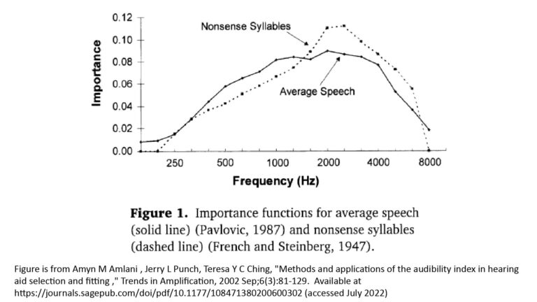
Fortunately, I’ve answered that question in part 1 of this series: if we have to pick a single frequency at which to predict the range of a typical directional microphone, it should be 2 kHz. That won’t yield a very accurate range prediction, but it will be close enough for many purposes.

However, there are still two other limitations of the DI approach:

• Some long-range microphones (like parabolic and horn microphones) provide gain as well as directivity, whereas the DF approach considers only directivity.
• For the same reason, the DF approach can’t account for differences in microphone self-noise between the subject directional microphone and the reference non-directional microphone, or for differences in the ambient noise.

Despite these issues, there are circumstances in which the DF approach yields useful range predictions. Specifically, it’s appropriate for microphones that have only modest directivity and no acoustic gain (such as shotgun microphones and studio microphones with cardioid-family polar patterns).

Using the DF: an example

Here’s an example of how a DF-based range prediction might be useful. Suppose you’re a videographer who needs to capture good-quality sound at a range of about 6 feet, and you’re considering the purchase of a Shure VP89L shotgun microphone for that purpose.

However, the VP89L costs about 1200 dollars, and you’d like to have some confidence that it will do what you expect it to do before you spend that much money.

From this figure of my post on how shotgun microphones work, you know that the VP89L will have a DI of about 10 dB at 2 kHz, which translates to a DF of 3. That means that it will have about 3 times the range of an isotropic microphone with the same self-noise under the same conditions.

Since you intend to use the VP89L at 6 feet, you now know that the signal quality will be about the same as with an isotropic microphone at 2 feet.

So, you can get a good idea of the VP89L’s signal quality in your application by positioning any reasonably quiet isotropic microphone (such as a good lavalier mic) 2 feet away from the source in the same environment in which you expect to use the VP89L.

A better way to predict microphone range: the SINR approach

As I explain in part 1 and part 2 of this series, the Signal-to-Interference-plus-Noise Ratio (SINR) is the best basis for quantifying the quality of a microphone’s output signal. And, unlike the DF, the SINR comprehends all of the factors that affect output signal quality, not just directivity. This makes it a much better basis for predicting microphone pick-up range.

As I explain in part 2, there are basically two SINR-based ways to quantify the quality of a microphone’s output signal, and this leads to two different approaches for SINR-based prediction of relative range.

The single-SINR approach to range prediction

As I explain in this section of part 2, we can get a reasonably good estimate of the quality of a microphone’s output signal via the SINR in an octave-wide sub-band centered at 2 kHz.

You can use this 2 kHz SINR to predict range by rearranging the SINR equation to solve for range as a function of SINR, and then plugging-in the minimum SINR required for the intended application. For example, I use 8 dB for applications (such as surveillance) in which poor fidelity is acceptable as long as voice remains at least 70 percent intelligible.

Alternatively, suppose you’ve already recorded sound with another reference microphone in the same environment in which you expect to use the subject microphone, and you know the maximum range at which it can provide an acceptable signal. You can calculate the SINR for that acceptable signal, and then solve for the range at which the subject microphone will provide the same SINR.

The multiple-SINR approach to range prediction

As described in detail in part 2, an even better measure of signal quality can be obtained by combining multiple SINR values evaluated for different sub-bands. At least two quality metrics can be obtained this way: one optimized for applications that stress high fidelity (which I call the Fidelity Index, or FI), and another for applications that stress voice intelligibility (which I call the Intelligibility Index, or II).

Either of these quality metrics can be used to predict microphone range in the same way as in the single-SINR approach described above. The only difference is that we can’t easily rearrange the expressions for either of these multiple-SINR quality metrics to solve for range. Instead, I use the goal-seek function in a spreadsheet to iteratively calculate the range at which the desired signal quality is achieved.

Comparing the results of the various range-prediction methods

The accuracy of any method of predicting microphone range is ultimately limited by the fact that signal quality is subjective. One person might feel that method A yields more accurate range predictions, while another might prefer method B. Reliably determining the “best” method of predicting microphone range would entail a lot of testing with many different individuals, which I haven’t yet done (and don’t have the resources to do).

On the other hand, I’m satisfied that the FI and II metrics I’ve developed are the “best” ones on which to base predictions of microphone range, at least for my purposes: they’re the most comprehensive and seem to yield the most accurate projections.

However, they’re also the most complicated, so it’s worth trying to determine if the differences are worth the added complexity. To that end, the following section compares the results of microphone range predictions using various methods and attempts to explain the differences.

Microphones for comparison

An important application for any method to predict microphone range is in evaluating the performance of long-range microphones. Therefore, I’m going to use the typical long-range microphones listed in the following table as a basis for the comparison, along with an isotropic microphone as a reference:

Type	Description	Notes
Isotropic	Non-directional microphone element with self-noise of 14 dBA	Bare microphone element used as reference for comparison. Same microphone element is also assumed in the exemplar long-range microphones listed below.
Parabolic	12-inch dish with dish efficiency of 0.6	Typical size of a DIY parabolic microphone using a solar-cooker dish
Parabolic	26-inch dish with dish efficiency of 0.6	Typical of commercially-available parabolic microphones; largest parabolic mic that isn’t prohibitively difficult to handle
Shotgun	12-inch interference tube with hypercardioid element	Typical of modern long shotgun mics (such as the Shure VP89L) which use a hybrid hypercardioid/interference-tube arrangement
Shotgun	24-inch interference tube with pressure mic element	Typical of a long DIY shotgun or machine-gun mic that isn’t prohibitively difficult to handle and does not include a hypercardioid element
Array	16-element array with 0.33-inch spacing	Represents the largest DIY array mic (in terms of number of elements) that’s still relatively easy to build; can achieve an extremely low self-noise using relatively inexpensive microphone elements.
Horn	12-inch exponential Acoustic Pressure Horn (APH)	Small DIY horn microphone using an inexpensive off-the-shelf speaker horn
Horn	32-inch conical Acoustic Pressure Horn (APH)	Large DIY horn microphone using an off-the-shelf cheerleader’s megaphone

Note that all of the microphones in Table 1 assume the same microphone element self-noise of 14 dBA.

Source level and ambient-noise assumptions

To facilitate microphone analysis, I’ve developed a set of target sound and ambient noise scenarios that I use for SINR estimation and range-prediction; these are documented in Predicting microphone performance—Part 1: what is SINR?

The range comparisons provided below are based on what I call the “general” scenario, which assumes that we want to pick-up human voice at a normal conversational volume (with an SPL of 70 dBA at 1 foot) in a reasonably quiet indoor environment (35 dBA broadband).

Comparing the Directivity Factor (DF) approach with the single-SINR approach

As I’ve already explained, the conventional DF approach to microphone range prediction is capable only of estimating the relative range of a directional microphone compared to an otherwise identical non-directional microphone—and only under exactly the same conditions and at a single frequency. On the other hand, the single-SINR approach considers all of the variables that influence SINR (but still at only a single frequency).

To illustrate the difference between these two approaches, the following chart shows two predicted ranges for each of the exemplar microphones:

• The first range is obtained using the “8 dB SINR at 2 kHz” method, where the 8 dB represents the minimum SINR for 70-percent voice intelligibility.
• The second range is the DF-predicted range: it’s the product of the DF at 2 kHz and the range of the isotropic micrphone using the “8 dB SINR at 2 kHz” method.

Here are the results:

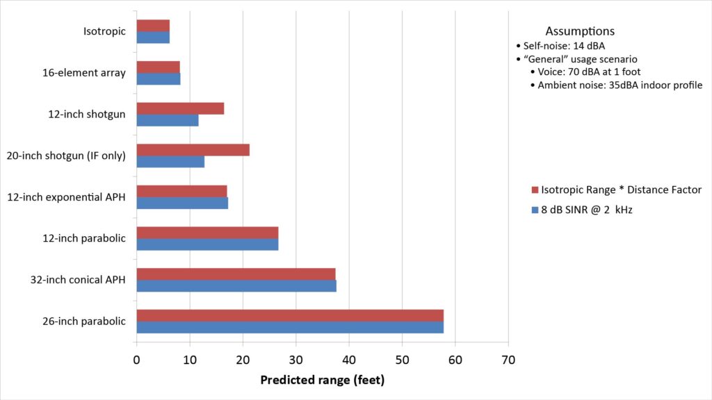
By definition, the range predictions for each method are identical for the isotropic microphone. The two range predictions are also almost (but not quite) identical for all of the other microphones except the shotgun microphones.

Here’s why: the shotgun microphones do not provide any acoustic gain, but they have enough directivity at 2 kHz to reduce the ambient noise term in the SINR to the point where it begins to approach the self-noise term. However, only the 8 dB SINR method comprehends the effects of self-noise; the DF doesn’t. Hence the DF over-predicts the range for the shotguns.

On the other hand, the other directional microphones provide substantial gain in addition to directivity. The gain is significant enough to keep the self-noise term well below the ambient noise term. As a result, the overall noise is dominated by ambient noise, and the DF is almost as accurate as the SINR in predicting the range.

As another example of the differing capabilities of the two methods, let’s consider another exemplar microphone: a 12-inch shotgun microphone with a self-noise of 21 dBA (instead of the 14 dBA of the original shotgun mic). The following chart shows the ranges predicted using the two methods for both the “noisy” and original shotgun microphones:

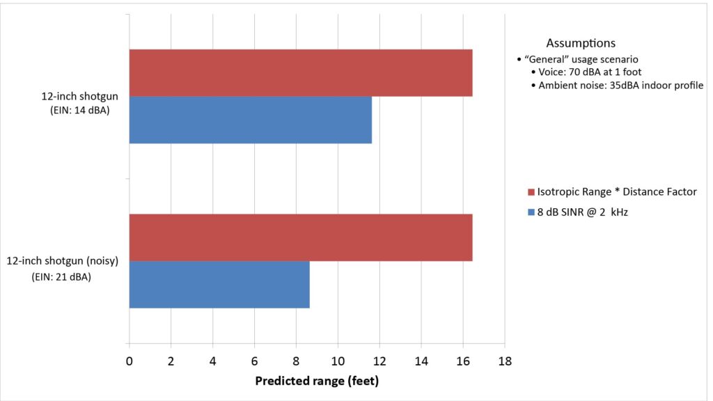
Of course, the ranges predicted by the DF method are the same for both microphones, since the method doesn’t address self-noise. The SINR method, however, shows how the increased self-noise decreases the range.

Comparing the single-SINR approach with the multiple-SINR approach

While the single-SINR approach does comprehend all of the variables that affect microphone range, it does so at only a single frequency. As a result, it can’t comprehend changes in the spectra of the desired sound and ambient noise, or variations in the frequency dependence of directivity and gain. That’s why I developed the Fidelity Index (FI) and Intelligibility Index (II).

As described in detail in Predicting microphone performance—Part 2: using the SINR, the FI and II are microphone signal-quality metrics based on the SINRs in 11 octave-wide frequency sub-bands.

Signal quality versus range using the FI and II

Before we compare range predictions from the single-SINR method with those based on the FI and II, let’s look at how the FI and II vary with range for the exemplar microphones in our “general” usage scenario:

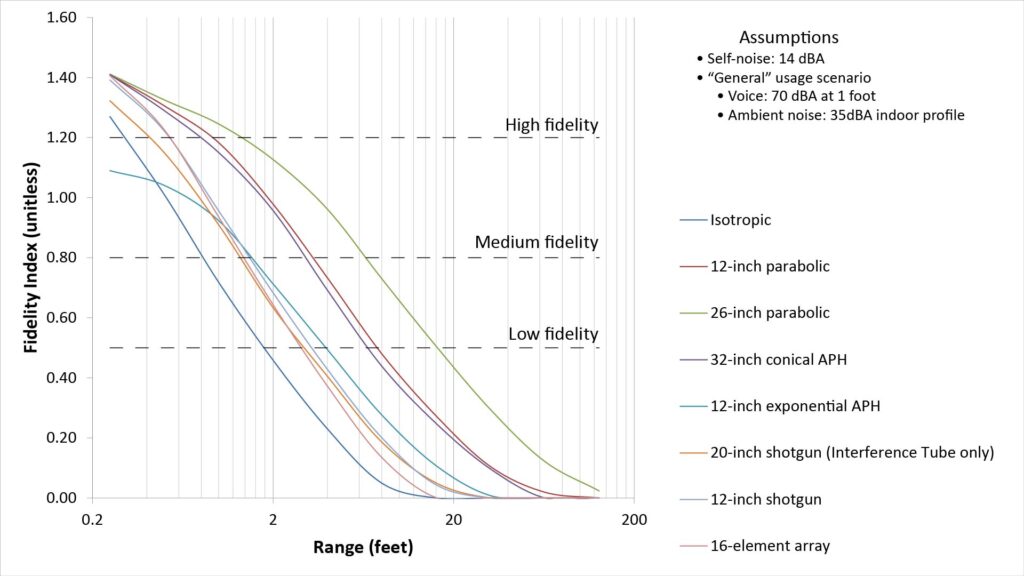
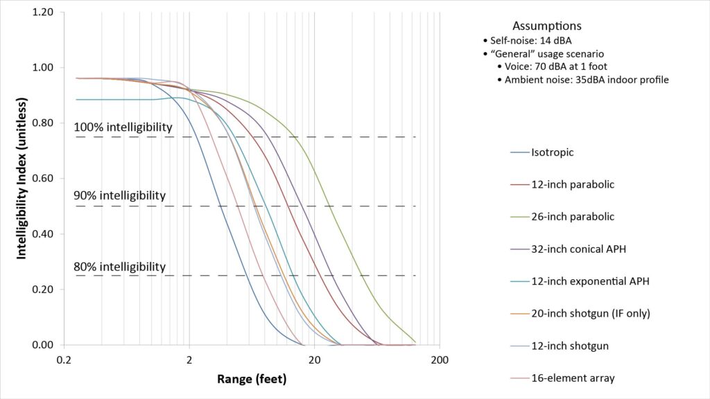
Note that each figure is labeled with three signal-quality thresholds, which I derived as described in the aforementioned post.

These curves indicate both the absolute and the relative ranges of the microphones:

• Absolute range is indicated by the X-axis value that corresponds to the desired signal quality on the Y-axis. The three signal-quality thresholds facilitate range prediction for various applications. However, signal quality is subjective, so there is some uncertainty in these thresholds and thus in the predicted absolute ranges.
• At any given level of signal quality, the ratio of the X-axis values for any pair of curves indicates the relative range between the corresponding pair of microphones. So, if you know that a particular microphone provides an acceptable signal quality at a certain range, you can use this method to find the range at which a different microphone can provide the same signal quality. This relative range ratio is analogous to the conventional Distance Factor, but is much more more useful for two reasons:
  • It comprehends all of the variables that determine microphone range (including acoustic gain, self-noise, source spectrum, and ambient noise spectrum), and not just directivity.
  • The relative range ratio is fairly invariant with signal quality. For example, if the curves indicate that microphone B provides twice the range of microphone A, that range ratio doesn’t vary much for different levels of signal quality. That mitigates some of the uncertainty due the subjective nature of signal quality.

Note that we could generate a similar signal-quality-versus-range curve using the 2 kHz SINR versus range, and we could define additional 2 kHz SINR thresholds (beyond the previously cited 8 dB) for various applications.

Maximum range versus signal quality

For most purposes, it will be more useful to predict the maximum range for the desired signal quality (as in Figures 2 and 3) than to plot the predicted signal quality versus range as in Figures 4 and 5.

The following figure shows four predicted ranges for the exemplar microphones; one obtained via the “8 dB SINR at 2 kHz” method, one using the FI, and two using the II:

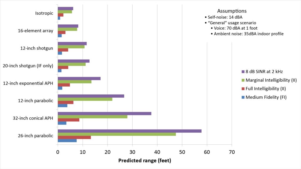
As we would expect, the predicted ranges increase as the required signal quality decreases.

The greatest range is predicted by the “8 dB SINR at 2 kHz” metric. However, note that the difference between this range and the ranges predicted by either the IF or II increases as a function of the microphone directivity:

• For the isotropic and 16-element arrays (which have no directivity and modest directivity, respectively), the 8 dB/2 kHz range is about the same as the “marginal intelligibility” range predicted using the II metric.
• However, the range difference is significant for the other microphones, all of which have significant directivity. That’s because the directivity of these microphones varies with frequency, and the 2 kHz SINR doesn’t reflect that fact.

Conclusions

In this post I’ve described three basic ways of predicting microphone range:

• the conventional Distance Factor (DF) approach;
• the “single SINR” approach, which involves finding the maximum range at which the SINR in single octave-wide sub-band (such as one centered at 2 kHz) is no less than some minimum acceptable value (such as 8 dB); and
• the “multiple SINR” approach, which involves finding the maximum range at which a multiple-SINR quality metric is no less than some minimum acceptable quality threshold.

The DF approach is the easiest but can’t comprehend the effects of anything but microphone directivity, and is therefore inappropriate for general-purpose microphone range predictions.

The single-SINR approach is more complicated but also much more useful than the DF, because it comprehends all the variables that can affect microphone range. However, because it’s based on the SINR in only a single frequency sub-band, it’s not appropriate for predicting the ranges of microphones that exhibit strong variation of directivity or gain with frequency—and that includes parabolic, shotgun, and horn microphones.