How array microphones work

An array microphone, sometimes called a microphone array, consists of multiple microphone elements whose outputs are electronically processed to provide a greater Signal-to-Noise Ratio SNR) and a sharper polar pattern than the individual elements.

There’s a lot of information online about array microphones (and array sensors in general), but most of it is theoretical and math-intensive. If you want a more intuitive understanding of how array microphones work—and especially if you’re interested in building one yourself—this post is for you.

A brief introduction to array microphones

An array microphone consists of an array of microphone elements whose outputs are electronically processed to provide a greater Signal-to-Noise Ratio SNR) and a sharper polar pattern than the individual microphone elements. The greater the number of microphone elements in the array, the greater the SNR gain and the sharper the polar pattern.

Array microphone configuration

A useful array microphone can have as few as a couple of microphone elements, but array microphones with thousands of elements have also been built.

Array microphone processing can be done in the analog or digital domain. It can be as simple as just summing the outputs of the microphone elements, or it can include time-delaying and amplitude-weighting of the microphone outputs before summing. Depending on the processing, an array’s polar pattern can be electronically steered to different directions without having to physically move the array, and there can even be multiple array outputs, each with its own polar pattern pointed in a different direction.

Array microphones exploit the principle of wave interference

Array microphones exploit the principle of wave interference: when two or more waves interact, they constructively or destructively interfere, depending on their relative phases.

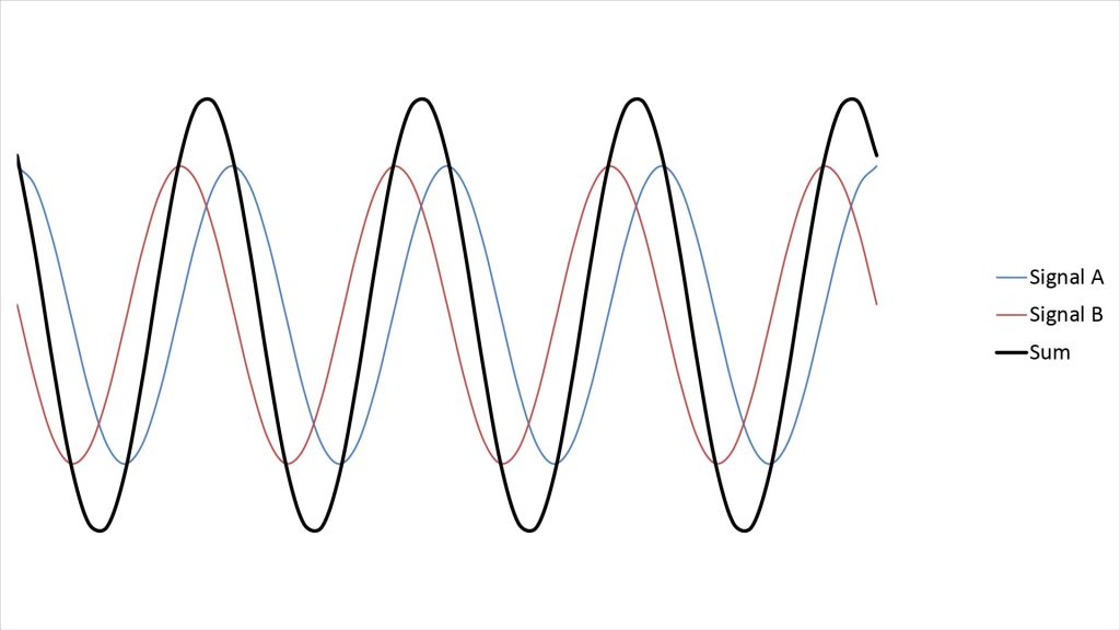
For example, if two sinusoidal signals of the same amplitude, frequency, and phase interact, they will constructively interfere to produce a sinusoid of the same frequency but twice the amplitude. But if the original sinusoids are 180 degrees out of phase, they will destructively interfere, canceling each other out. Intermediate phase differences (but with the same frequency) will yield intermediate amplitudes, as shown in the example in the accompanying figure.

In an array microphone, the outputs of the individual microphones are the signals whose interference is exploited, and the interference occurs electronically in the array processing.

And here’s how array microphones exploit wave interference: phase differences between the microphone signals are caused by sound reaching the microphones at slightly different times, depending on the direction of sound arrival and the physical arrangement of the microphones.

So, sounds arriving from desired directions experience constructive interference, while sounds arriving from other directions experience destructive interference. Optionally, the directions in which constructive and destructive interference occur can be adjusted by time-delaying the microphone signals to alter their phases prior to further processing.

Array microphone figures-of-merit

Before we get into how array microphones work, let’s review four key figures-of-merit that are helpful in characterizing the performance of array microphones: SNR gain, Array Factor (AF), directivity, and on-axis frequency response.

Signal-to-Noise Ratio (SNR) gain

The Signal-to-Noise Ratio (SNR) gain of an array microphone is the increase in the SNR of the array, over the SNR of its individual microphones, in an intended direction of maximum sensitivity (referred to as an on-axis direction).

Notice that the definition above refers to “an” intended direction, not “the” intended direction. That’s because array microphones can provide maximum sensitivity in different directions at the same time.

The maximum SNR gain of an array microphone increases with the number of microphone elements. Depending on the type of array, the SNR gain can also be frequency-dependent.

Be aware that the term “array gain” is also used in connection with array microphones; this sometimes refers to what is described here as SNR gain, but sometimes refers to what is described below as the Directivity Index.

The Array Factor (AF)

One of the key benefits of an array microphone is that it provides a sharper polar pattern than its constituent microphone elements, which in turn enhances the rejection of off-axis noise.

The polar pattern of an array microphone is equal to the product of the polar pattern of the individual microphone elements and what is called the array’s Array Factor (AF). The AF is always frequency-dependent, but the way it varies with frequency depends on the array configuration.

Because the array’s polar pattern is the product of its AF and the microphone pattern, the AF also represents the polar pattern the array would have if its constituent microphones had an isotropic polar pattern. Thus, if an array actually does use isotropic (pressure-type) microphone elements, then its polar pattern will be the same as its AF.

The polar pattern of an individual microphone usually represents its power pattern, which is the square of its voltage (or amplitude) pattern. Similarly, the square of the AF is what is typically used to characterize an array’s directional characteristics.

Therefore, the AF is usually presented as a polar plot of 20logAF (which represents the square of the AF in dB) versus off-axis angle in a given plane, like the polar pattern plots provided by microphone manufacturers. Unless otherwise stated, all of the AF charts on this site also plot the power response (AF squared), not the voltage response (AF).

Here’s an example of an AF plot for a hypothetical array designed to capture sounds arriving from zero degrees:

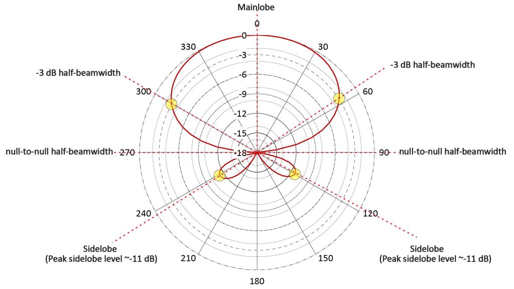
The peaks in the AF are referred to as lobes. The full-power lobe in the intended direction of maximum sensitivity (at zero degrees) is called the mainlobe, while the lesser lobes in other directions are called sidelobes. By the way, AF plots aren’t always oriented so that the intended direction of maximum sensitivity is at zero degrees, and some arrays are designed to have more than one direction of maximum sensitivity (so that they have more than one mainlobe).

Sometimes, there are additional full-power lobes at directions other than the intended direction(s) of maximum sensitivity (although the pattern in Figure 2 doesn’t have them); these are called grating lobes. Whether a full-power lobe is considered a mainlobe or a grating lobe depends on the purpose of the array.

As shown in Figure 2, an array’s AF can be characterized by metrics such as beamwidth and peak sidelobe level:

• The beamwidth is the angular extent of the AF in the on-axis direction over which the power response is no less than some specified value. A typical value is -3 dB, and the corresponding beamwidth is referred to as the Half-Power BeamWidth (HPBW), which is about 115 degrees for the pattern of Figure 2.
• Another beamwidth measure is the null-to-null beamwidth, which is the width between the mainlobe nulls (about 180 degrees for the pattern of Figure 2).
• The peak sidelobe level is the level of the sidelobe with the highest peak. Sometimes there are multiple peak sidelobes, such as the two peak sidelobes of about -11 dB of Figure 2.

Because the AF gives the polar pattern in just a single plane, two AFs in orthogonal planes (such as vertical and horizontal) may be necessary to fully characterize an array’s directional characteristics in two dimensions. We’ll discuss AFs much more later in this post.

Directivity (D) and Directivity Index (DI)

The two benefits of an array microphone—SNR gain for sounds arriving from an on-axis direction, and improved rejection of off-axis sounds due to the Array Factor—can be comprehended in just a single metric: directivity.

The directivity D of an array microphone (or any directional sensor) is defined as the ratio of its on-axis power response to its average power response over all directions. It’s most often quantified as the Directivity Index (DI), which is just the ratio D in dB: DI = 10log(D). So, for example, an isotropic (pressure-type) microphone has a D of 1 and a DI of 0 dB, because its on-axis response is equal to its average response over all directions.

Because the DI of an array depends on its AF, it is always frequency-dependent…but the way in which it varies with frequency depends on the type of array.

The DI is an extremely useful metric because it represents the performance gain provided by the array in the presence of isotropic noise (noise which reaches the microphone with equal power from all directions). Actual noise is almost never truly isotropic, but isotropic noise is a good approximation for the noise in many situations in which an array microphone could be useful.

For example, consider the problem of recording voice in a room with a lot of hard surfaces. Reverberations from those surfaces can be considered to be reasonably isotropic noise. If the microphone’s polar pattern is also isotropic, then it must be placed very close to the person speaking to keep the reverberations from being audible in the recording…and that’s not always possible. A directive microphone aimed at the source allows the microphone to be placed further from the source, because its directivity compensates for the inverse-square losses caused by increasing the microphone-to-source distance.

Depending on the number of elements and the type of processing, an array microphone can provide a DI considerably greater than the 6 dB of a hypercardioid microphone.

On-axis frequency response

In the same way that an array microphone modulates the polar response of its constituent microphone elements, it also modulates their frequency response.

So, while the frequency response of its individual microphones might be flat, the on-axis frequency response of some types of array can have both a low-frequency roll-off and high-frequency fluctuations due to aliasing effects.

The fundamental array microphone building-block: the two-element array

With a basic introduction out of the way, we can get into more detail on how array microphones work.

Because array microphones work on the principle of wave interference, and because only two waves are necessary for wave interference to occur, an array microphone can be built with as few as two microphone elements.

In fact, the operation of any array microphone, no matter how complex, can be analyzed by examining the phase differences between the signals from a pair of adjacent microphone elements.

So we’ll start our look at array microphones by examining the fundamental array-microphone building-block, which is a simple two-element array. This could be a stand-alone array microphone, or a portion of a larger array microphone. A block diagram of such a two-element array microphone is shown in Figure 3:

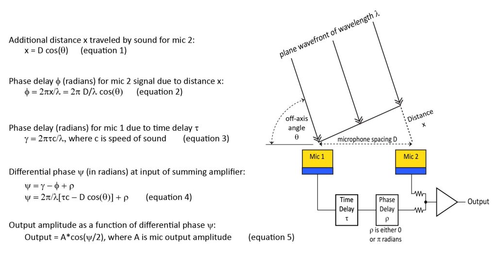
This array consists of a pair of identical microphone elements separated by a distance D. The elements are pressure-type microphones which have an isotropic polar pattern (not all array microphones use pressure-type microphone elements, but many do; we’ll discuss why later).

The output of microphone 2 is connected directly to an input of a summing amplifier. On the other hand, the output of microphone 1 goes through two processing stages before being reaching the same summing amplifier:

• The first stage is a time delay of τ seconds.
• The second stage is a phase delay of ρ radians. For the purposes of our discussion, ρ can have just one of two values: zero or π radians. Note that setting p to pi radians is equivalent to multiplying the signal by -1, which is also equivalent to putting an inverting amplifier in the signal path or replacing the summing amplifier with a differential amplifier.

This array can be made to operated in different ways by changing τ and ρ, as we’ll soon see.

The key to array operation: differential phase

As shown in Figure 3, both microphones are receiving sound in the form of a plane wavefront of wavelength λ, which is tilted by an angle θ such that the sound has to travel further to reach mic 2 than mic 1.

The key to the operation of this two-element array is the differential phase ψ between the signals at the input of the summing amplifier. As expressed by equation 4 in Figure 3, ψ is a function of the the microphone spacing, the tilt θ and wavelength λ of the incoming wave, the time delay τ, and the phase delay ρ.

And once we know the differential phase ψ, we can find the amplitude of the array output as the sum of the two microphone signals, using equation 5.

SNR gain of the two-element array

Suppose that the variables of equation 4 are such that the differential phase ψ is zero. Then, according to equation 5, the array output amplitude will be twice the microphone signal amplitude (representing an amplitude gain of 3 dB).

But since power is proportional to the square of the amplitude, the signal power at the array output will be greater than the microphone signal power by a factor of four, or 6 dB.

Unfortunately, the microphone signals will also contain a noise component due to the microphone self-noise. However, unlike the signal component due to incident sound, each microphone’s self-noise is random and independent. Therefore, because there is no correlation between the noise signals, the noise amplitudes don’t add, but the noise powers do. So the noise power at the array output will be twice the noise power in each microphone signal, for a power gain of 3 dB.

Thus, this two-microphone configuration has a peak SNR gain of (6 – 3) dB, or 3 dB, which occurs when ψ is zero. The gain will decrease as ψ increases, becoming infinitely small at π radians or 180 degrees, and then increase again as ψ approaches 360 degrees.

Array Factors of the two-element array

We can also use equations 4 and 5 of Figure 3 to plot the Array Factor (AF) of the array as a function of off-axis angle θ.

However, note that for a given wavelength λ and microphone spacing D, the differential phase ψ at the summing amplifier depends not just on the the off-axis angle θ, but also on the time delay τ and phase delay ρ.

In fact, we can drastically change the behavior of our two-element array by adjusting τ and ρ. We can bound the range of possible behaviors by the four configurations shown in Figure 4:

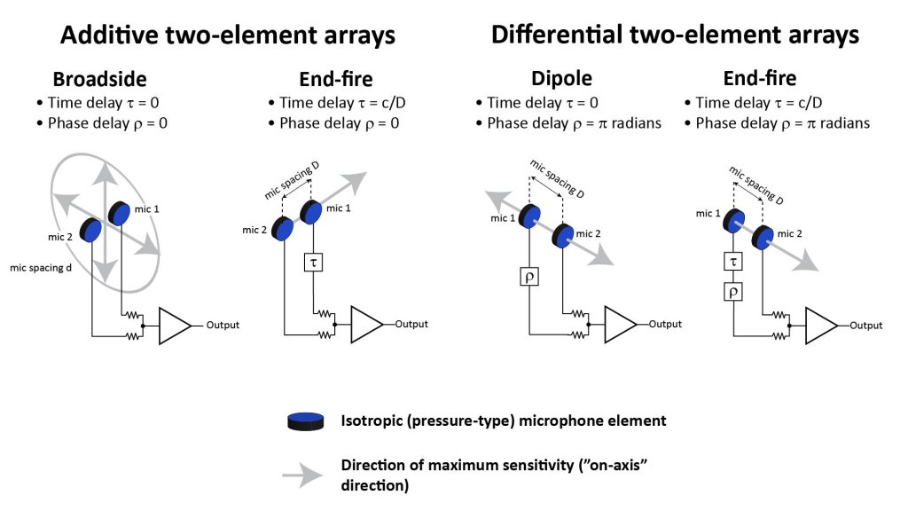
• If the phase delay ρ is set to zero, the array operates as an additive array: the output is the sum of the microphone signals (one of which is optionally time-delayed).
• If the phase delay ρ is set to pi radians, the array operates as a differential array: the output is the difference of the microphone signals (one of which is optionally time-delayed).
• Changing the time delay τ changes the shape of the array’s AF in a way that depends on whether the array is operating as an additive or differential array.

Each of the four configurations of Figure 4 has many applications, so we’ll discuss each separately.

Two-element additive broadside array microphone

First we’ll consider the left-most array of Figure 4, which has the time delay τ and phase delay ρ both set to zero.

For this array, the differential phase ψ between the inputs to the summing amplifier will also be zero—causing a peak in the AF—for sound coming from a direction perpendicular to a plane containing the centers of the microphone diaphragms.

An array designed to have maximum sensitivity in a direction perpendicular to the plane of its elements is called a broadside array. Incidentally, the term “broadside” has its roots in early naval artillery, when guns were mounted on the sides of ships so that the direction of fire was perpendicular to the ships’ lengths.

Note that, for any two element array, the microphone locations are always colinear, so there is an infinite number of planes containing the centers of the microphone diaphragms. Thus, rather than a single on-axis direction, a linear broadside array actually has a circle of on-axis directions. If there were three or more elements, they could be arranged as a planar array (in which all the element locations are co-planar but not colinear) or a volumetric array (in which all the elements are not co-planar), which we’ll discuss later.

Looking at the diagram of the broadside array in Figure 4, it’s obvious that sound arriving from the broadside direction will reach both microphones in-phase regardless of the sound’s wavelength. This means that this additive broadside array has a flat on-axis frequency response, and the same is true of all additive arrays.

How about this array’s response in other directions? We’ll look at a plot of its AF shortly, but first let’s consider the response to sound traveling along the line connecting the microphones:

• If the wavelength of the sound is twice the microphone spacing, then the microphone signals will be 180 degrees out of phase and will cancel completely, causing a null in the response.
• But if the sound’s wavelength is equal to the spacing, the outputs will be in-phase, causing a full-power peak in the response (which, as noted above is called a grating lobe).

This illustrates the main issue with additive arrays: while they have a flat on-axis frequency response, the off-axis response—and therefore the shape of the AF—is frequency dependent.

We can see that more clearly by using equations 4 and 5 of Figure 3 to plot the AF versus off-axis angle θ at four different frequencies, assuming a microphone spacing of one inch.

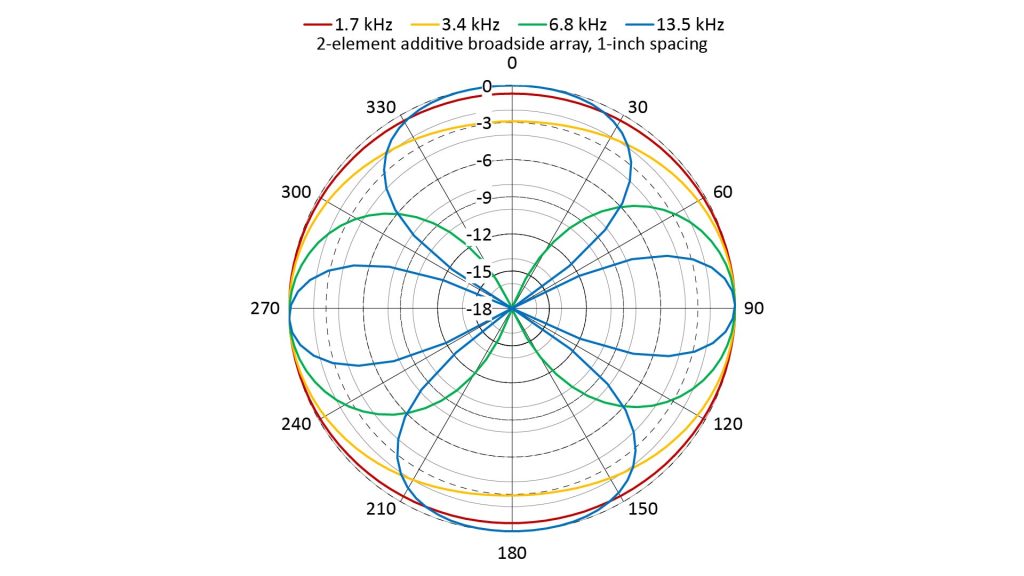
Notice that, at all four frequencies, there are peaks at 90 and 270 degrees, which is where we would expect the mainlobes to be for broadside aiming. However, the off-axis response is clearly frequency-dependent:

• At 1.7 kHz, the microphone spacing is just one-eighth of a wavelength. So the differential phase for sounds arriving from 0 or 180 degrees isn’t enough to cause significant cancellation. As a result, the AF factor is almost omnidirectional, so that the DI is barely greater than 0 dB. All two-element additive arrays have limited directivity at frequencies at which the microphone spacing D is much smaller than a wavelength.
• The AF becomes more directional at 3.4 kHz (D=0.25λ), and still more directional at 6.8 kHz (D = 0.5λ): the mainlobes get sharper and the nulls at 0 and 180 degrees get deeper.
• But at 13.5 kHz (D= 1.0λ), the nulls at 0 and 180 degrees have been replaced by broad grating lobes, seriously degrading the directivity.

In fact, an additive broadside array has maximum directivity when the microphone spacing is equal to half a wavelength. Grating lobes appear above that frequency, while at lower frequencies the mainlobes get broader and the nulls get shallower.

Two-element additive end-fire array microphone

The additive end-fire array shown in Figure 4 is exactly like the additive broadside array, except that the output of the first microphone is time-delayed before the summing operation, and the time delay τ is equal to the time needed for sound to travel between the microphones.

This will cause the inputs to the summing amplifier to be perfectly in-phase for sound traveling in the direction from microphone 1 to microphone 2, so that the array output will be equal to twice the microphone outputs. Hence, the on-axis direction points from microphone 2 toward microphone 1, or at θ= 0 degrees. This is called end-fire aiming.

As with the additive broadside array, the on-axis direction of the additive end-fire array doesn’t depend on the wavelength of the sound, so the on-axis frequency response is flat.

Now consider sounds arriving from from 180 degrees off-axis (traveling in the direction from microphone 2 to microphone 1). The sound will reach microphone 1 after a delay of τ, and microphone 1’s output will be electronically delayed by another τ before it reaches the summing amplifier. Thus, there will be a net delay of 2τ between the signals at the input of the summing amplifier. The phase difference caused by this delay, and hence the output of the amplifier, will depend on the wavelength of the sound:

• When the wavelength is much longer than the microphone spacing D (say by a factor of ten), the 2τ delay will result in only a small phase difference between the signals at the input of the summing amplifier. The array output will then be almost twice that of the microphone outputs, and thus almost equal to the on-axis peak. Thus, we can see that this two-element additive end-fire array provides little off-axis rejection of wavelengths that are long compared to the microphone spacing.
• As the wavelength gets shorter, the phase difference begins to increase, causing the amplifier output to drop. When the wavelength has dropped to 4D, the 2τ delay will result in a differential phase of a half wavelength (180 degrees), causing the signals to cancel. Thus, this two-element additive end-fire array provides near-perfect rejection at 180 degrees at a wavelength of four times the microphone spacing (and harmonics thereof). At this wavelength, the pattern is a unidirectional cardioid.
• As the wavelength gets shorter than 4D, the differential phase starts to increase past 180 degrees, so the array output begins to rise again. When the wavelength has dropped to 2D, the 2τ delay results in a differential phase of 360 degrees, causing the signals at the input of the amplifier to once again be in-phase. Thus, this two-element additive end-fire array has no rejection at 180 degrees at a wavelength of twice the microphone spacing (and harmonics thereof).

The upshot is that, like the additive broadside array, the additive end-fire array’s ability to reject off-axis noise is frequency-dependent.

This is further evident in the following figure, which shows the AFs for the two-element additive end-fire array at the same frequencies and for the same microphone spacing as the broadside array:

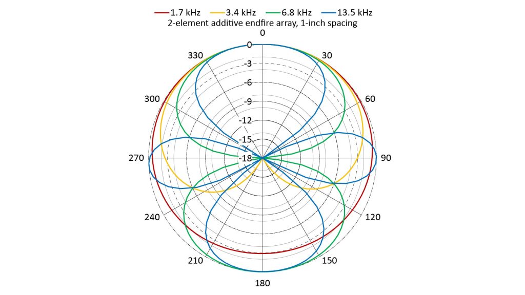
Notice that there is now only one direction where the peaks for all four frequencies line-up, so there is now only one mainlobe…and that mainlobe is at zero degrees, versus the two mainlobes at 90 and 270 degrees for the broadside array. In fact, we can steer the array between broadside and end-fire aiming by varying τ between zero and D/c seconds.

Another difference between the end-fire and broadside arrays is that maximum directivity (just short of the onset of grating lobes) occurs at a microphone spacing of 0.25λ, instead of 0.5λ as for the broadside array. Because the end-fire array has only one mainlobe instead of two, we would also expect its maximum DI to be greater than that of the broadside array, and in fact its peak DI is twice that of the broadside array (6 dB versus 3 dB).

However, the additive end-fire array has the same problem as the additive broadside array: it directivity drops both above and below the frequency at which the microphone spacing is 0.25λ:

• Grating lobes appear at higher frequencies. At 6.8 kHz (D=0.5λ), the AF becomes bidirectional, so the end-fire has lost its directivity advantage over the broadside array. At 13.5 kHz, there are now three grating lobes and the directivity has dropped still further.
• At 1.7 kHz (D=0.25λ), the rejection at 180 degrees is only 3 dB.

Incidentally, a shotgun microphone works exactly like an additive end-fire array, except that it uses slots instead of microphone elements, and the distance from each slot to the microphone diaphragm provides the time delay. See my post on how shotgun microphones work for much more detail on shotgun mic operation.

Two-element differential dipole array microphone

If the phase delay ρ is set to π radians but the time delay τ is left at zero, we get the third configuration shown in Figure 4. Setting ρ to π radians is equivalent to inverting the signal from microphone 1, so the array output is effectively the difference between the two microphone signals. This makes the configuration a Differential Microphone Array (DMA), and the fact that there is no time delay gives it a dipole (bidirectional) pattern. Here’s why:

Sounds arriving from a direction perpendicular to the line between the microphones will arrive at each microphone in-phase. But since the outputs are subtracted, rather than added, these in-phase signals cancel, causing a deep null in that direction (instead of the peak we’d get with an additive broadside array). In fact, a differential dipole array will have a deep null perpendicular to the line containing the microphone at all wavelengths.

Now consider sound traveling from one microphone toward the other (in either direction). Unlike sounds arriving perpendicularly to the line connecting the microphones, the response in these directions will depend on the wavelength:

• When the wavelength is much longer than the microphone spacing (say by a factor of ten), then the differential phase at the input of the amplifier will be small, and the subtraction operation will result in a very small output. A differential array has a poor on-axis response at wavelengths much longer than the microphone spacing.
• As the wavelength gets shorter, the differential phase increases, causing the amplifier output to also increase. When the wavelength has dropped to twice the microphone spacing (2D), the differential phase is 180 degrees, and the subtraction operation causes the array output to be twice that of the microphone outputs. Thus, there is a response peak in the AF. A differential dipole array provides a perfect dipole (bidirectional) pattern, like a ribbon microphone, at a wavelength equal to twice the microphone spacing (and harmonics thereof).
• As the wavelength gets shorter still, the differential phase passes 180 degrees on its way to 360 degrees, and the array output begins to fall. When the wavelength has reached the microphone spacing D, the inputs to the differential amplifier are in-phase again, and the array output is zero. A differential dipole array always has an on-axis null at a wavelength equal to the microphone spacing (and harmonics thereof).

The following figure shows the the AFs for the differential dipole array at the same frequencies as for the other arrays, and assuming the same one-inch microphone spacing:

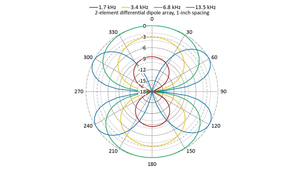
Notice that the peaks for the three lower frequencies line-up at 0 and 180 degrees; these are the dipole mainlobes. But unlike the mainlobes of the additive broadside array (FIgure 5), these mainlobes are frequency-dependent: they get smaller at lower frequencies, and get replaced by off-axis grating lobes when the microphone spacing exceeds a half-wavelength (13.5 kHz, D=1.0λ). All differential arrays have a low-frequency roll-off and aliasing at higher frequencies.

Also like the additive broadside array, there are two nulls (in this case at 90 and 270 degrees). But unlike the nulls of the broadside array, these nulls don’t get shallower as the frequency decreases.

In fact, unlike the AF of the broadside array, the AF of the differential dipole maintains its shape (and directivity) at frequencies at which the microphone spacing is less than a half-wavelength.

Two-element differential end-fire array microphone

The fourth and final type of two-element array shown in Figure 4 is equivalent to the differential dipole array, except that the time delay τ is now changed from 0 to D/c (the time required for sound to travel from one microphone to the other).

Unlike the two-element additive arrays, changing the time delay in a differential array doesn’t steer the mainlobe(s), but rather steers the nulls. Recall that the differential dipole array (Figure 7) had mainlobes at both 0 and 180 degrees, but adding a time delay of D/c puts a null at 0 degrees, turning the dipole pattern into an end-fire pattern.

Here’s why. Consider sound arriving from 180 degrees off-axis (traveling from microphone 1 toward microphone 2). Because the delay τ is equal to the time required for the sound to travel between the microphones, the positive and negative inputs of the differential amplifier will see exactly the same signal, so the array output is zero. A differential end-fire array always has a null at 180 degrees, and this null is independent of wavelength.

Now consider sounds arriving from the on-axis (opposite) direction, traveling from microphone 2 toward microphone 1. Because of the time delay τ, the signal from microphone 2 will be delayed by 2τ relative to the signal from microphone 1. The differential phase caused by this 2τ delay, and hence the output of the differential amplifier, will depend on the wavelength of the sound:

• When the wavelength is much longer than the microphone spacing (say by a factor of ten), then the differential phase at the input of the amplifier will be small, and the subtraction operation will result in a very small output. Like a differential dipole array, a differential end-fire array has a poor on-axis response at wavelengths much longer than the microphone spacing.
• As the wavelength gets shorter, the differential phase increases, causing the amplifier output to also increase. When the wavelength has dropped to 4D, the total time delay of 2τ will cause a differential phase of 180 degrees, so the subtraction operation causes the array output to be twice that of the microphone outputs. Thus, a differential end-fire array has an on-axis peak at a wavelength equal to four times the microphone spacing (and harmonics thereof).
• As the wavelength gets shorter still, the differential phase passes 180 degrees on its way to 360 degrees, and the array output begins to fall. When the wavelength has reached 2D, the inputs to the differential amplifier are in-phase again, and the array output is zero. A differential end-fire array always has an on-axis null at a wavelength equal to twice the microphone spacing (and harmonics thereof).

The following figure shows the the AFs for the differential end-fire array at the same frequencies as for the other arrays, and assuming the same one-inch microphone spacing:

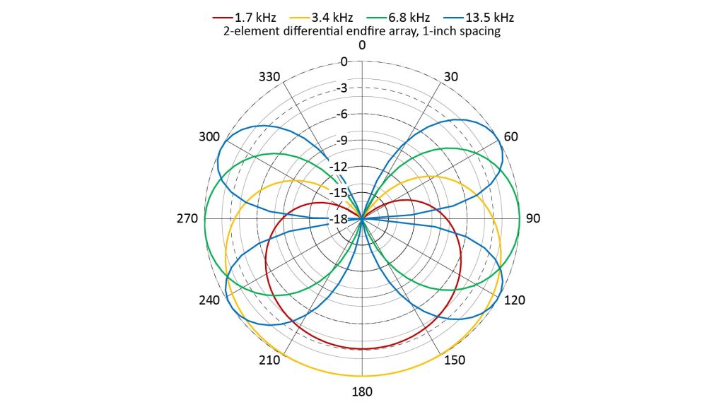
Notice that the peaks for the two lower frequencies line-up at 180 degrees; this is the end-fire mainlobe. Like the two mainlobes of the differential dipole array (Figure 7), this mainlobe is frequency-dependent: it gets smaller at lower frequencies. Also like the differential dipole array, this differential end-fire array exhibits aliasing in the AF—but this aliasing occurs at frequencies for which the microphone spacing is greater than 0.25λ, rather than 0.5λ.

Finally, like the differential dipole array, and unlike the additive arrays, the shape of the AF doesn’t change at frequencies below which aliasing occurs.

Directivity of two-element array microphones

Before we discuss actual Directivity Indices (DIs), we can make some qualitative observations about the directivity of the various two-element arrays by inspecting the AFs of Figures 5 through 8.

First, it’s obvious that the directivity of all four types of array degrades in the presence of grating lobes. So the following discussion will assume operation at frequencies below which grating lobes occur.

Additive broadside array versus differential dipole array

First, let’s compare the AFs of the two arrays with bidirectional patterns: the additive broadside array (Figure 5) and the differential dipole (Figure 7).

When the microphone spacing is a half-wavelength (which occurs at 6.8 kHz with a one-inch spacing), they both have two full-power mainlobes and no sidelobes. However, the broadside array’s mainlobes have a -3 dB beamwidth of about 60 degrees, while those of the differential dipole have a -3 dB beamwidth of 120 degrees.

Does that mean that the additive broadside array has greater directivity?

No, because as depicted in Figure 4, the additive broadside array is directive in just one plane, while the differential dipole is directive in two orthogonal planes. If we plotted the AF of the additive broadside array in an orthogonal plane, it would be omnidirectional, whereas the AF of the differential dipole array would be the same.

In fact, at a spacing of a half-wavelength, the additive broadside array and the differential dipole array have exactly the same directivity.

However, at lower frequencies, the AF of the additive broadside array starts looking more omnidirectional, while the AF of the differential dipole array retains its shape. In fact, below the aliasing frequency, the directivity of an additive array decreases with frequency, while that of differential arrays remains constant.

Additive end-fire array versus differential end-fire array

Unlike the additive broadside array (but like the differential end-fire array), the additive end-fire array is directive in two orthogonal planes. And by comparing the AF of the additive end-fire (Figure 6) to that of the differential end-fire (Figure 8), we can see that they have exactly the same cardioid pattern when the microphone spacing is exactly a quarter-wavelength.

So it would appear that they have the same directivity at this microphone spacing—and, in fact, they do. But, again, the directivity of the additive array drops with frequency, while that of the differential array remains constant.

Broadside/dipole directivity versus end-fire directivity

Intuitively, the end-fire arrays should be more directive than the additive broadside and differential dipole arrays, because the former have one mainlobe but the latter have two. In fact, they are more directive: the peak directivity of both two-element end-fire arrays is twice that of either the additive broadside or differential end-fire array.

Peak Directivity Indices (DIs) of the two-element arrays

Now let’s expand our directivity discussion with some numbers.

We know from our discussion above that, below the frequency at which aliasing occurs, the directivity of additive arrays decreases with decreasing frequency. But that raises two questions:

• What is the peak Directivity Index (DI) of the additive two-element arrays, and how does it compare with the peak DIs of the differential arrays?
• Under exactly what conditions does the peak DI occur?

It turns out that the peak directivity of array microphones is determined just by the number of elements and the mainlobe steering direction (between broadside and end-fire), and not the type of array (additive versus differential). The peak DIs for an N-element array are as follows:

• Broadside (both additive and differential dipole): DI = 10log(N), or 3 dB for a two-element array.
• End-fire (both additive and differential): DI=10log(N^2), or 6 dB for a two-element array.

For broadside aiming, this peak directivity occurs at the frequency at which the microphone spacing is exactly one-half wavelength for additive arrays, and at and below that frequency for differential arrays.

However, the conditions under which the peak DI occurs for end-fire aiming is a bit less straightforward.

maximum directivity for end-fire aiming requires hypercardioid pattern

The most directive AFs shown in Figures 6 and 8 have a pure cardioid pattern. However, end-fire arrays are also capable of producing other cardioid-like patterns that have slightly greater directivity than pure cardioids. Two of the most useful of these are the supercardioid and hypercardioid patterns, which (along with the pure cardioid) are shown in the figure below:

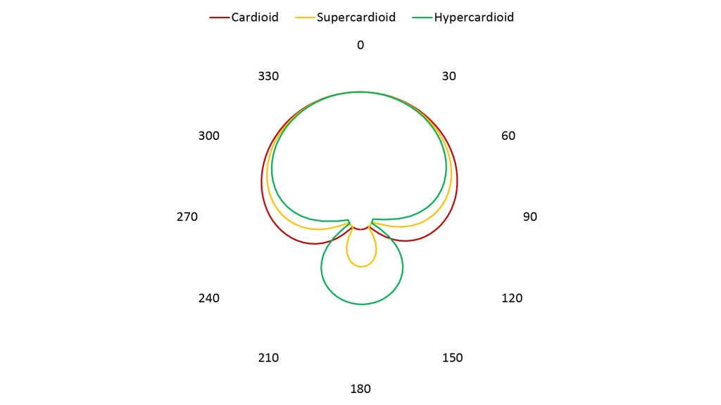
The supercardioid and hypercardioid have narrower mainlobes than the cardoid, but at the expense of sidelobes at 180 degrees. Both have a greater DI than the pure cardioid; the hypercardioid offers the maximum DI achievable with a two-element array, while the supercardoid offers the greatest front-to-back ratio achievable with a two-element array.

So the peak DI given by the formula above is achievable only with the hypercardioid pattern. But how do we get a hypercardoid pattern? That depends on the type of end-fire array.

For the two-element additive end-fire array, the supercardioid and hypercardioid patterns occur only at specific frequencies slightly greater than the frequency at which a cardioid pattern is obtained. The super- and hypercardioids are the result of slight aliasing in the pattern (well short of the aliasing that would cause grating lobes). We can see that in the AF plots below (again assuming a one-inch microphone spacing):

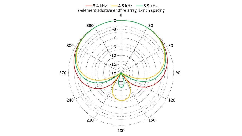
Of course, because this is an additive array, the patterns become more omnidirectional at lower frequencies.

For the differential end-fire array, the cardioid pattern also begins to look more like a supercardioid, and then a hypercardioid, as the frequency is increased slightly. However, the differential end-fire array offers another, much better, way to achieve a supercardioid or hypercardioid pattern: by changing the time delay:

• When τ=D/c, the pattern is a cardioid.
• When τ=D/(0.707c), the pattern is a supercardioid.
• When τ=D/2c, the pattern is a hypercardioid.

We can see that in the following AFs, all at 3.4 kHz and assuming a one-inch spacing:

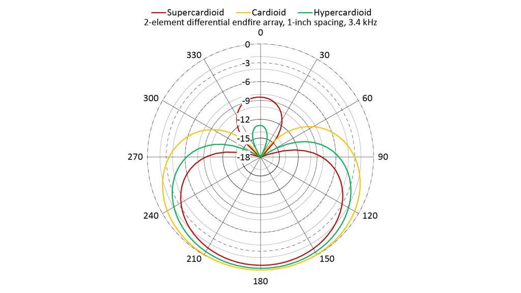
And as we already know, unlike the additive end-fire, the differential end-fire array maintains these patterns at lower frequencies.

Frequency response of two-element differential array

As we’ve discussed, differential arrays—unlike additive arrays—have a non-flat frequency response.

Specifically, the response is aliased at frequencies above the frequency at which grating lobes occur, and it has a 6-dB-per-octave roll-off below that frequency. And the SNR gain is degraded in exactly the same way as the frequency response.

We can see this graphically by using the same equations we used to plot the AF versus angle (equations 4 and 5 of Figure 3) to plot the on-axis AF versus frequency. The following figure shows the on-axis frequency response of the two-element differential end-fire array for three different values of microphone spacing D:

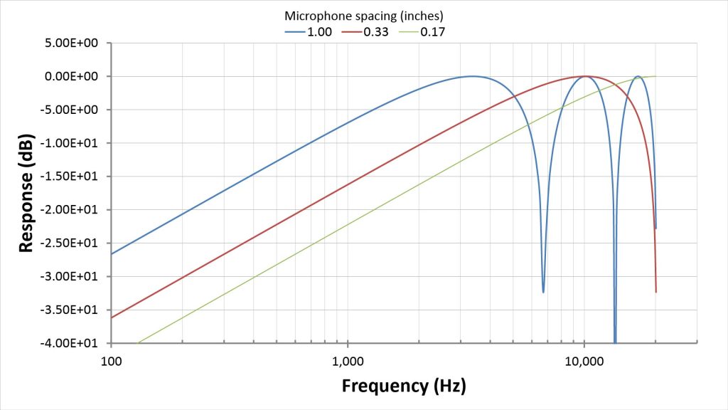
These curves illustrate the main issue with differential arrays: limited operating bandwidth:

• At the upper end, the bandwidth is limited by the frequency at which aliasing begins (which, for end-fire aiming, is the frequency at which the microphone spacing is a quarter wavelength).
• At the lower end, the bandwidth is limited by the 6-dB-per-octave low-frequency roll-off. We can electronically boost the lower frequencies to equalize the response, but there is a limit to the boost we can apply. That’s because equalization will also amplify the microphone self-noise at those frequencies.

We can raise the aliasing frequency by reducing the microphone spacing…but then we would need even more low-frequency equalization:

• With a microphone spacing of one inch, the upper limit on bandwidth is just 3.4 kHz.
• We can increase this to about 20 kHz by decreasing the spacing to 0.17 inches…but then the required equalization at, say, 300 Hz has doubled from a manageable 17 dB to a probably-unmanageable 33 dB.

Similarities between differential array microphones and conventional studio microphones

Before we wrap-up our discussion of two-element arrays, let’s examine the parallels between the two-element differential array microphones and studio microphones with which you might be familiar.

Pressure-gradient microphones operate like differential dipole arrays

In a two-element differential dipole array, the output is obtained by subtracting two electrical signals (or, equivalently, by adding one electrical signal to another signal that has been phase-shifted by π radians, as shown in Figure 4).

The same thing happens acoustically with a single microphone whose diaphragm is open on both sides, because such a diaphragm responds to the difference in the pressures across the diaphragm. This is exactly how bidirectional studio microphones work (although they sometimes use ribbons rather than diaphragms), and why they are sometimes called pressure-gradient microphones.

But why don’t pressure-gradient microphones suffer from the problem of limited bandwidth we discussed above for differential arrays? Actually, they do suffer from limited bandwidth, but they incorporate design features to mitigate the problem:

• As we’ve discussed, aliasing in the frequency response of a differential array occurs when the microphone spacing becomes greater than a certain fraction of a wavelength (0.5 wavelengths for a dipole and 0.25 wavelengths for end-fire aiming). In a pressure-gradient microphone, the analogous distance is the acoustic path length across the diaphragm. This acoustic path length is typically much smaller than the one-inch spacing we assumed for our notional array, so such a pressure-gradient microphone will be able to operate at a much higher frequency without aliasing.
• However, as we’ve noted, the smaller the microphone spacing in a differential array, the poorer the response at low frequencies due to its inherent 6-dB-per-octave high-pass characteristic. The same effect happens with a pressure-gradient microphone—and the loss is much worse due to the relatively short acoustic path length. But rather than electronically boosting the low frequencies, a pressure-gradient microphone equalizes the response by exploiting the fact that the mass of a microphone diaphragm causes a 6-dB-per-octave low-pass characteristic. By carefully adjusting the diaphragm mass, this low-pass effect can be made to exactly compensate the high-pass effect due to wave interference…resulting in a nearly-flat frequency response.

Differential dipole arrays can use analogous techniques to mitigate their inherent limitations: microphone spacing can be reduced to raise the aliasing frequency, and an electronic high-pass filter (or low-frequency amplification) can be used to equalize the response.

Cardioid-type microphones operate like differential end-fire arrays

We’ve seen that a two-element differential dipole array can be turned into an end-fire array by electronically time-delaying one of the two electrical signals before they’re subtracted. Cardioid, supercardioid, and hypercardioid patterns (or anything in-between) can be obtained by varying the time delay.

Similarly, a pressure-gradient microphone can be turned into a cardioid, supercardioid, or hypercardioid microphone by acoustically time-delaying the sound reaching one side of the microphone diaphragm. And the same math regarding the relationship between the time delay and the pattern applies to both differential arrays and pressure-gradient-based microphones.

There are also parallels in the way the time delays can be implemented in the electrical and acoustic domains. One way of implementing an electrical time delay is to discretely time-sample the signal and then clock it through a shift register of the required length; analogously, an acoustic time delay can be implemented by passing sound wave through a transmission line of the required length. In fact, that’s how the earliest cardioid microphones were built: sound reached one side of the diaphragm directly, but had to pass through a transmission line before reaching the other side.

Another way to implement an electrical time delay is use an all-pass filter, which exploits the fact that a time delay is equivalent to a frequency-dependent phase shift. This enables a time delay to be implemented using only capacitors, inductors, and resistors (although active all-pass filters that don’t require inductors are more practical than purely passive filters). Similarly, an all-pass filter can be implemented acoustically using the acoustic analogs of capacitors, inductors, and resistors.

However, purely acoustic implementations of cardioid-type microphones are less flexible than differential end-fire arrays, and arguably more difficult to build for the DIY microphone enthusiast.

Two-element array theory explains the proximity effect

Studio microphones that use some type of pressure-gradient microphone capsule can exhibit what is known as the proximity effect: a dramatic boosting of low frequencies when the sound source is placed close to the mic.

Most online discussions of the proximity effect describe what it is and under what circumstances it occurs, but not what causes it. The array theory we’ve been discussing provides the explanation:

• As we’ve seen, a pressure-gradient microphone capsule behaves like a two-element differential array: the output is equal to the difference between the sound pressures on each side of the diaphragm.
• Sound arriving from in front of the microphone has to travel a slightly longer distance to reach the back of the diaphragm than to reach the front of the diaphragm. As we’ve seen, this differential acoustic path length causes a 6-dB-per-octave low-frequency roll-off. In a well-designed studio mic, this is compensated by a 6-dB-per-octave high-frequency roll-off due to diaphragm mass, resulting in a near-flat response.
• However, for all this to work properly, the sounds reaching each side of the diaphragm must experience almost exactly the same attenuation. This is the case when the distance from the source to the microphone is much larger than the differential acoustic path length between the front and back of the diaphragm.
• But as the sound source gets closer to the microphone, the differential acoustic path length starts becoming a significant fraction of source-to-microphone distance. The sound reaching the back of the diaphragm then begins to experience significantly greater attenuation than the sound reaching the front of the diaphragm. Now, sounds that should cancel completely (such as 90-degree off-axis sound in the case of a bidirectional capsule, or 180-degree off-axis sound in the case of a cardioid capsule) don’t cancel completely, degrading the polar pattern.
• This incomplete cancellation also means that the low frequencies no longer roll-off at 6 dB per octave. In fact, when the source is very close to the front of the microphone, the low-frequency roll-off can essentially disappear. However, the 6-dB-per-octave high-frequency roll-off due to diaphragm mass remains, which is what causes the bass-heavy characteristic known as the proximity effect.

Limitations of two-element array microphones

We began our discussion of array microphones with simple two-element arrays primarily as a learning exercise, but some two-element arrays do have practical applications. Before we discuss those practical applications, let’s review some of the obvious limitations of two-element arrays:

• Modest peak directivity. Any type of two-element array has a maximum directivity of 6 dB (achieved with end-fire aiming and a hypercardioid pattern). This is enough to be useful in many applications, but many other applications that call for directional microphones (such as picking-up voice at long range) require much greater directivity.
• Limited directivity at low frequencies in the additive configuration. Additive arrays have the advantage of a flat on-axis frequency response and SNR gain, but become virtually isotropic (equally sensitive in all directions) when the microphone spacing is much shorter than a wavelength.
• Limited bandwidth in the differential configuration. Differential arrays retain their directivity at lower frequencies, but have high-frequency aliasing and a low-frequency roll-off that limits their usable bandwidth.

From the standpoint of practical applications, the most serious of these limitations is the limited low-frequency directivity of the two-element additive array. As we’ll see later, larger additive array microphones can be quite useful, but (in my opinion) a two-element additive array doesn’t provide enough advantage over a single microphone to be worth the trouble. Indeed, I’m not aware of any practical applications of two-element additive arrays.

Two-element differential array microphones, on the other hand, are quite useful. Their potential usefulness is demonstrated by the fact that all pressure-gradient (figure-eight) and unidirectional (cardioid, supercardioid, and hypercardioid) studio microphones operate on exactly the same principle as the two-element differential array.

Array microphones with more than two elements

All of the disadvantages of two-element arrays—the modest peak directivity, the limited low-frequency directivity of additive arrays, and the limited bandwidth for differential arrays—can be mitigated by increasing the number of microphone elements.

How increasing the number of elements improves array performance

From our discussion of two-element array microphones, we know that the microphone spacing is a trade-off:

• Increasing the spacing sharpens the polar pattern (for additive arrays) and improves the on-axis low-frequency response (for differential arrays).
• However, increasing the spacing also reduces the frequency at which aliasing occurs (manifested by grating lobes with additive arrays, or nulls in the on-axis frequency response with differential arrays).

Now, suppose that we have an N-element array microphone with a uniform microphone spacing of D, where N>>2. The signal from the first microphone will interfere with the signal from not only the second microphone, but also with the signals from all the other microphones in the array.

Viewing an N-element array as a superposition of virtual two-element arrays

Therefore, the output of an N-element array can be viewed as the superposition of the outputs of many virtual two-element arrays, each with a different inter-element spacing: there will be (N-1) virtual two-element arrays with a spacing of D, (N-2) virtual two-element arrays with a spacing of 2D, (N-3) virtual two-element arrays with a spacing of 3D, and finally one virtual two-element array with a spacing of (N-1)*D.

Let’s see the implications of this for both additive and differential arrays

Additive arrays as a superposition of virtual two-element arrays

If the N-element array is configured as an additive array, then each virtual array’s spacing will determine its mainlobe width, its maximum operating frequency without grating lobes, and the number and angular position of its grating lobes at a given frequency. The (N-1) virtual arrays with a spacing of D will have the broadest mainlobe but the highest aliasing frequency, while the one virtual array with a spacing of (N-1)*D will have the narrowest mainlobe but the lowest aliasing frequency (and the greatest number of grating lobes at a given frequency).

The mainlobes for all of these virtual arrays will line-up at the same angle. So their peaks will add, yielding an on-axis power gain of 20log(N) dB and an SNR gain of 10log(N) dB, while the combined mainlobe width will be the weighted average of the mainlobe widths of all the virtual arrays. Thus, adding elements to an additive array increases the gain and sharpens the mainlobe, with the mainlobe width being inversely proportional to longest microphone spacing.

But unlike the mainlobes, only grating lobes at certain angles will be common to all of the virtual arrays—and those will be the angles of the grating lobes corresponding to the smallest spacing D. So, those will be the only grating lobes in the combined array output that experience the full array gain. Meanwhile, grating lobes at other angles (corresponding to other values of microphone spacing) will experience less gain, and will thereby be attenuated and become sidelobes in the final array response. Thus, an N-element additive array retains much of the benefit of the relatively high aliasing frequency of the shortest microphone spacing, due to attenuation of the lower-frequency grating lobes corresponding to the longer spacings.

So, adding elements to an additive array microphone gives the best of both worlds: the mainlobe sharpness of a longer microphone spacing, but with the relatively high aliasing frequency of a shorter microphone spacing. We’ll see this graphically when we discuss the Array Factors (AFs) for some N-element additive arrays later on in this post.

Differential arrays as a superposition of virtual two-element arrays

Additional elements affect a differential array’s frequency response in much the same way they affect an additive array’s polar response.

If the N-element array described above is configured as a differential array, then each virtual two-element array’s spacing will determine the maximum frequency at which it can operate without aliasing, as well as its low-frequency response. The (N-1) virtual arrays with a spacing of D will have the highest alias-free operating frequency but the poorest low-frequency response, while the one virtual array with a spacing of (N-1)*D will have the lowest alias-free operating frequency but the best low-frequency response.

When the frequency responses for these virtual arrays are superimposed, only the aliased nulls at certain frequencies will be common to all of the virtual arrays—and those will be the frequencies of the nulls corresponding to the smallest spacing D. The nulls at other frequencies (corresponding to other values of microphone spacing) won’t line-up, and will thereby become shallower in the overall array response. Thus, an N-element differential array retains much of the benefit of the relatively high aliasing frequency of the shortest microphone spacing, due to the partial filling-in of nulls caused by the longer microphone spacings.

Meanwhile, all of the virtual arrays will contribute to the response below the lowest aliasing frequency.

Thus, adding elements to a differential array microphone gives the best of both worlds: the low-frequency response of a longer microphone spacing, but with the relatively high aliasing frequency of a shorter microphone spacing.

The downside to more elements: increased complexity

Of course, arrays with more elements are more expensive and complex to build. The least complex type of large array is the additive array with fixed broadside aiming. Because they don’t need time delays and require the fewest amplifiers, additive arrays with a dozen or more elements and fixed broadside aiming are relatively easy DIY projects.

However, with end-fire arrays (or any array with an electronically adjustable polar pattern), each additional element requires an additional time-delay (and, in the case of differential end-fire arrays, an additional amplifier). That’s illustrated in Figure 13 for three element arrays:

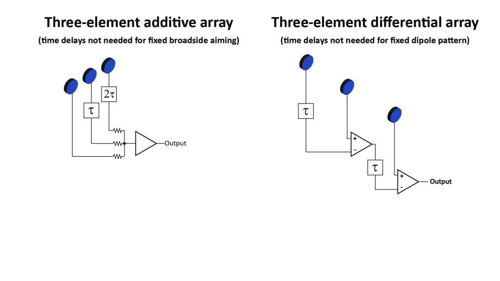
So, arrays that require time delays (and especially differential arrays) can quickly become prohibitively complex to implement as the number of elements is increased.

Differential arrays present another difficulty as the number of elements increases. Not only do they require an additional time delay and amplifier per element, but differential array microphones are extremely sensitive to any mismatch between the microphone elements or unwanted amplitude or phase shifts in the electronics…and this sensitivity increases with the number of elements.

At the same time, as we’ve discussed, differential arrays with just two elements (which work just like pressure-gradient and cardioid-type microphones) are already quite useful. For these reasons, differential array microphones with more that two elements are relatively rare, and I won’t spend too much time on them in this post.

Larger arrays can be linear, planar, or volumetric

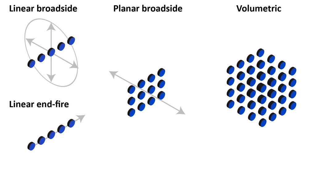
All two-element arrays are always linear arrays because any two objects in space can always be connected with a straight line. But arrays with a greater number of elements can also be planar or volumetric:

• If the elements are colinear (arranged in a line), the array is linear.
• If the elements are coplanar but not colinear, the array is a planar array.
• If the elements are not coplanar, the array is a volumetric array.

Examples of these configurations are shown in Figure 14.

Linear arrays

The two-element arrays we discussed previously are linear arrays because the centers of two elements are always colinear. Linear arrays in the additive end-fire or differential configurations provide directivity in two planes (like a flashlight beam), but linear arrays in the additive broadside configuration provide directivity in only one plane (like a fan beam).

For example, a horizontal linear broadside array (like that shown in Figure 14) would provide directivity only in the horizontal plane. Such an array would be useful in isolating the voice of a single person from many people sitting around a conference-room table, but would be ineffective at suppressing echoes from the ceiling or floor.

The only way to make an additive broadside array directive in two planes is to arrange the elements as a planar array.

Planar arrays

An additive planar array can provide directivity in two planes when steered to the broadside direction. Figure 15 shows an example of an additive planar array microphone, in this case a rectangular array of twelve microphones arranged as three rows by four columns.

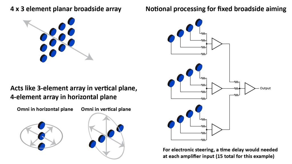
Each row can be considered to be a separate horizontal linear array whose four element outputs are processed to yield a single output for that row. The three row outputs are then processed as if they were the elements in a three-element vertical element array, to yield the overall array output.

This array behaves like a 4-element linear array in the horizontal plane, and like a 3-element linear array in the vertical plane. Therefore, the overall array polar pattern is fan-shaped, and directional in both the horizontal and vertical planes.

The array shown in Figure 15 is designed for fixed broadside aiming. If electronic steering of the mainlobe is needed, then a planar array requires a time delay for each element, plus a time delay for each row or each column.

Planar arrays have two Array Factors (AFs)

Because a planar array provides directivity in two orthogonal planes, it also has two AFs. If the array has the same number of elements (and element spacing) in each dimension, then the two AFs will be the same.

But an oblong planar array (one with a different number of elements along each axis), like that shown in Figure 15, will have a different AF in each plane. That’s illustrated in Figure 16:

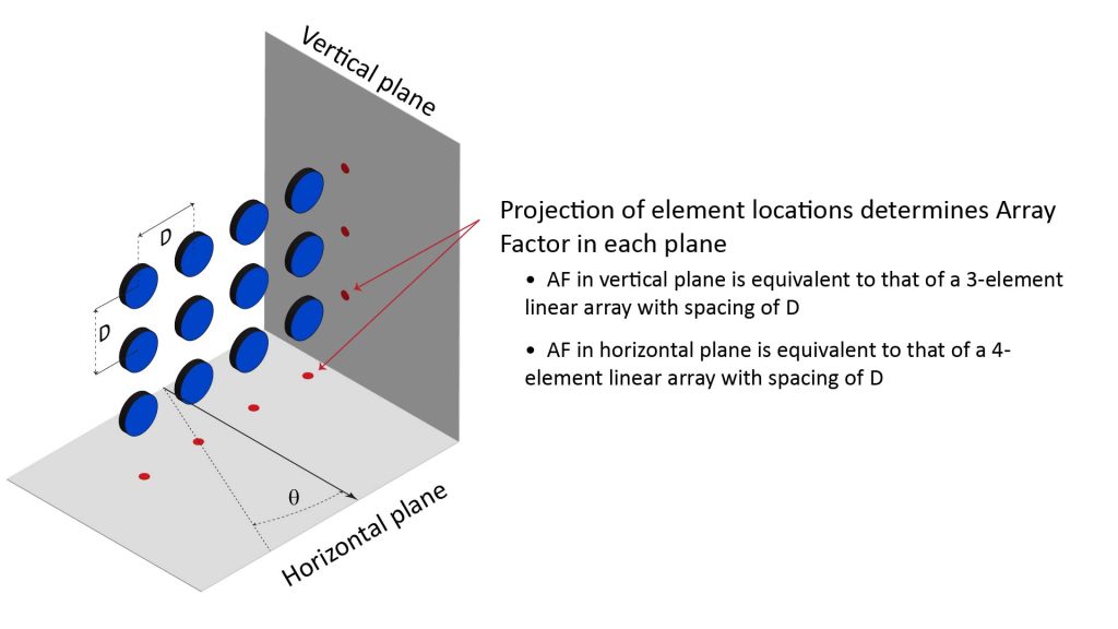
Thus, an N by M element planar array has the AF of a N-element linear array in one plane, and an M-element linear array in the orthogonal plane.

Volumetric arrays

A volumetric array is one in which the elements are not all coplanar.

An additive volumetric array is potentially capable of steering its mainlobe to any solid angle, providing spherical coverage. Such a capability can be extremely useful in applications such as advanced sonar systems for undersea surveillance. However, while based on the same physics as linear and planar array microphones, volumetric arrays are currently too complex to actually implement to warrant much attention in this post.

An exception is a relatively simple volumetric array consisting of two planar additive arrays (such as the array shown in Figure 15), each with fixed broadside aiming, whose outputs are processed as a two-element differential end-fire array. I’ll discuss such a configuration in an upcoming post, and design of a similar microphone is described in an Analog Devices application note [1].

SNR gain and Directivity Index (DI) of an N-element array microphone

The SNR gain and DI of an N-element array can be determined using the same formulas used for the two-element arrays we previously discussed:

• Peak on-axis SNR gain = 10log(N), where N is the number of microphone elements. This gain is flat with frequency for an additive array, but varies with frequency for a differential array. Note that it depends only on the number of elements, and not how they’re spaced or arranged.
• The peak DI for an array with broadside aiming is equal to 10log(2N∗S/λ), where N is the number of microphone elements, S is the element spacing, and λ is the wavelength. If the spacing is λ/2 (previously mentioned as optimum for a broadside array), then this reduces to DI = 10log(N), the same as the SNR gain. This DI is flat with frequency for a differential dipole array (below the frequency at which aliasing occurs), but drops with frequency for an additive broadside array. This peak DI is independent of the pattern in which the microphones are arranged.
• The peak DI for an array with end-fire aiming is equal to 10log(4N∗S/λ), where N is the number of microphone elements, S is the element spacing, and λ is the wavelength. If the spacing is λ/4 (previously mentioned as optimum for an end-fire array), then this reduces to DI = 10log(N), the same as the SNR gain. End-fire arrays are generally linear arrays, and we can also express the DI for a linear end-fire array whose length is much greater than the spacing (which is typically the case) as DI = 10log(4L/λ), where L is the array length. Again, the DI is flat with frequency for a differential end-fire array (below the frequency at which aliasing occurs), but drops with frequency for an additive end-fire array.

The Array Factor (AF) of an N-element array

A planar array has two AFs (and a volumetric array has three AFs). As illustrated in Figure 16 for a planar array, each AF is equivalent to the AF of a virtual linear array formed by the projection of the microphone elements in the corresponding plane. But how do we determine the AF of an N-element linear array?

Way back in our discussion of two-element arrays, we used equation 5 of Figure 3 to determine the array output as a sum of two phase-shifted sinusoids. Obviously, we can’t use that equation to determine the array output for an N-element linear array when N is greater than two.

AFs for N-element additive arrays

Fortunately, the math to determine the AF of a linear additive array of an arbitrary number of uniformly spaced and weighted colinear elements isn’t much more complicated than for just a pair of elements, provided that the array has uniform element spacing and equal amplitude weighting. The necessary math was worked out back in the 1930s when the first array radars and line microphones were conceived.

As with a two-element array, a key term in determining the AF of an additive array of N uniformly-spaced and equally-weighted colinear elements is the differential phase ψ between adjacent elements. The AF of such an N-element array is given by the following equation:

AF = Abs[(sin(Nψ/2))/(Nsin(ψ/2))] (equation 7), where ψ is the same differential phase given by equation 4 of Figure 3.

Now we can plot the AF of an additive array of an arbitrary number of uniformly spaced and equally weighted colinear elements, for both broadside and end-fire aiming.

By the way, we can also use equation 7 to plot the AF of a shotgun microphone, which works exactly like an additive end-fire array. See my post on how shotgun microphones work for a comparison of the AF plotted using equation 7 with the manufacturer-provided AF for a commercial shotgun mic.

Sample AFs for N-element additive array microphones

To illustrate the benefit of additional elements, we can can use equation 7 above to plot the AFs for several additive linear arrays of varying size.

The following figure shows AF plots for additive linear broadside arrays with 2, 4, and 16 elements, with a microphone spacing of a half-wavelength (0.33 inches at 20 kHz):

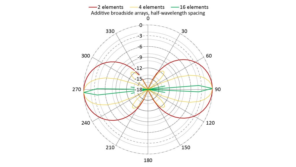
All three arrays have a bidirectional pattern, as we would expect with broadside aiming.

The two-element array has the widest mainlobes and no sidelobes (as we would expect for a microphone spacing of a half-wavelength).

Note that the four-element array’s mainlobes are only half the width of those of the two-element array. This is because the spacing between the first and fourth microphones is twice the spacing of the two-element array (a full wavelength versus a half-wavelength). If this were a two-element array, a spacing of one wavelength would result in full-power grating lobes, but in this four-element array the grating lobes have been reduced to sidelobes of only about -11 dB.

For the 16-element array, the mainlobe gets even narrower (by a factor of four), and the sidelobes have dropped to -13 dB from the four-element array’s -11 dB. In fact, for uniformly spaced and equally-weighted arrays much larger than 2 elements, the peak sidelobe level is always about -13 dB. By the way, there are also other sidelobes in this array’s pattern, but they are below the minimum plot scale of -18 dB.

The following figure shows AF plots for additive linear end-fire arrays with 2, 4, and 16 elements, with a microphone spacing of a quarter-wavelength (0.33 inches at 10 kHz):

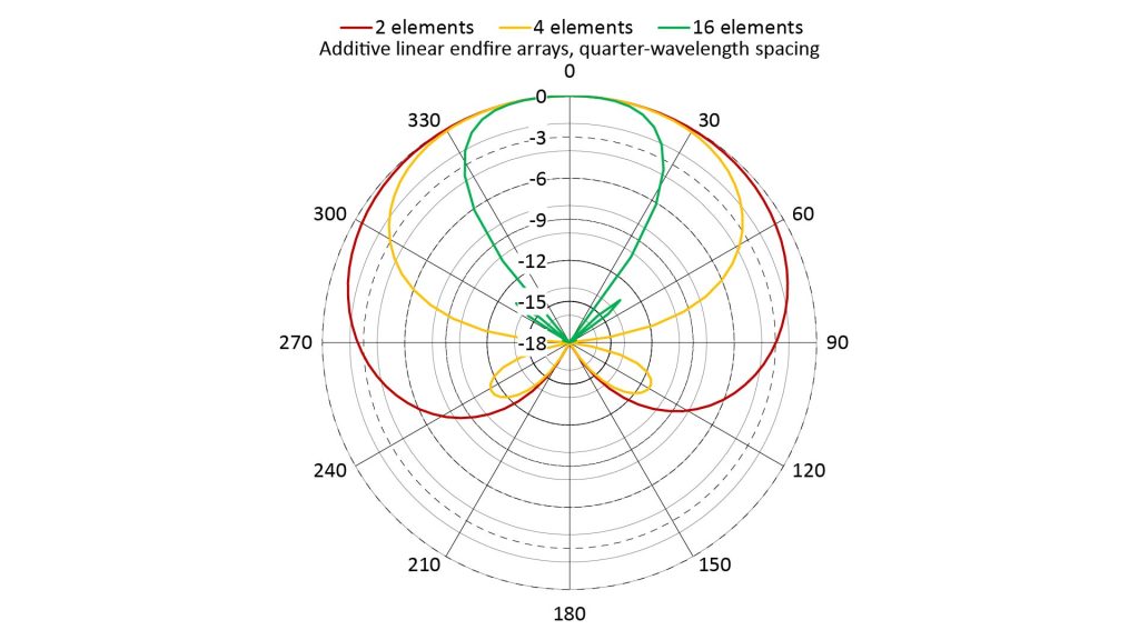
As with the broadside arrays, the mainlobes of the end-fire arrays get narrower as the the number of elements increases, and instead of grating lobes there are much smaller sidelobes.

Of course, because these are additive arrays, grating lobes would appear at frequencies above the frequency at which the microphone spacing is a half-wavelength (for the broadside arrays) and a quarter-wavelength (for the end-fire arrays).

AFs for N-element differential arrays

Unfortunately, I haven’t yet found a simple formula (like equation 7 above for additive arrays) to determine the AF of an N-element differential array.

On the other hand, I haven’t found the need for such a formula, either, for two reasons:

• Because differential arrays with more than a few elements are difficult to implement (especially due to their extreme sensitivity to mismatch between the microphone elements and signal paths), I don’t plan on building one soon.
• If there are only a few elements, it’s easy to build a spreadsheet that uses equation 5 of Figure 3 to sum the outputs of each stage of an N-element differential array to determine the array factor numerically.

However, this post is already about three times the size I had intended, and I have to draw the line somewhere…so I’m not going to include any sample AFs for larger differential arrays.

Array microphones versus other directional microphones

As we’ve seen, array microphones with just a few elements can provide useful directivity; for example, cardioid, supercardioid, or hypercardioid patterns can be achieved with just two elements.

However, tens or even hundreds of elements are needed to obtain enough directivity to pick up sounds at long ranges, and as previously discussed, such an array microphone can be extremely complex and expensive.

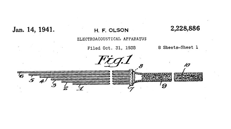
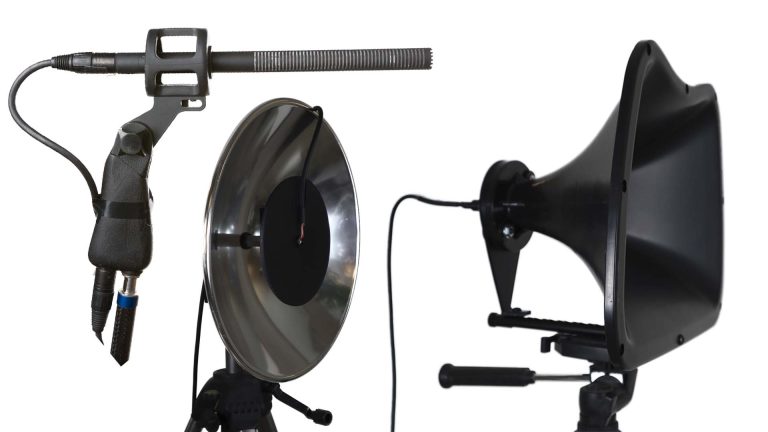
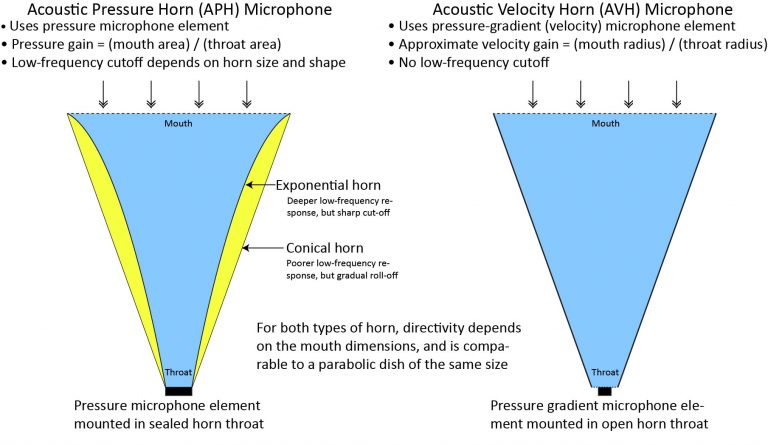
So, at least from a DIY perspective, array microphones aren’t practical alternatives to parabolic, shotgun, or horn microphones for picking-up sound at long ranges. See this comparison in my post on long-range directional microphones for more info on that topic. And check out the following posts if you’re interested in microphones offering very high directivity:

• How parabolic microphones work
• How shotgun microphones work
• How horn microphones work

Wrap-up

Hopefully, this post has given you a good overview of array microphones and how they work. But this site is all about DIY microphones, and if you’re interested in actually building a useful array microphone, check out the next post in this series: Practical DIY array microphones.

References

1. Analog Devices application note AN-1328, available at https://www.analog.com/media/en/technical-documentation/application-notes/AN-1328.pdf [accessed June 2021]. Describes principle of operation, design, and construction of professional grade studio or live performance microphone using up to 32 analog MEMS microphones connected to op amps and a difference amplifier. Design is a volumetric array consisting of two additive broadside arrays in a differential end-fire configuration.
2. TDK InvenSense applicaton note AN-1140, available at https://invensense.tdk.com/wp-content/uploads/2015/02/Microphone-Array-Beamforming.pdf [accessed June 2021]. Discusses basic principles and performance of various array configurations.
3. Iain McCowan, “Microphone Arrays : A Tutorial,” April 2001, available at http://www.aplu.ch/home/download/microphone_array.pdf [accessed June 2021]. Detailed, math-intensive treatise on array microphones.
4. Sverre Holm, “Differential arrays – from cardioid microphones to Yagi antennas,” Department of Informatics, University of Oslo, available at https://www.mn.uio.no/fysikk/english/people/aca/sverre/lecturenotes/2020-differentialarrays-cardioid-yagi.pdf [accessed June 2021]. Extremely useful and understandable reference on differential microphone arrays.