The 4 key microphone specifications and why they’re important

A microphone’s performance in any given application will be determined mostly by just four key microphone specifications. In this post I’ll explain what they are, why they’re important, and how to choose them for a given application.

The purpose of microphone performance specifications

The ideal microphone would produce an output signal that’s the perfect analog of the sound reaching it: the output would have exactly the same spectral characteristics as the sound and wouldn’t contain any added distortion or noise. Further, the ideal microphone would respond only to the sounds we want to capture while ignoring sounds we don’t want to capture.

Unfortunately, the ideal microphone doesn’t exist. We can get close to ideal behavior in some areas, but only if we’re willing to compromise in others.

That’s where performance specifications come in: by quantifying the degree to which each aspect of a microphone’s performance lives up to the ideal, they help us achieve the best compromise for a given application.

The “big four” microphone performance specifications

In any given application, a microphone’s overall performance will be mostly determined by just three key specs:

• The maximum distortion-free Sound Pressure Level (SPL)
• The Effective Input Noise (EIN), sometimes called self-noise and sometimes specified implicitly via the Signal-to-Noise Ratio (SNR)
• Polar response (which can be specified in several ways, the most appropriate of which depends on the application)
• Effective bandwidth (the range of frequencies over which the microphone’s output meets the other requirements)

Another spec—sensitivity—is also important, but generally has a minimal impact on overall performance as long as the device to which the microphone is connected has a relatively quiet input stage.

I’ll go over each of these in detail.

Maximum distortion-free SPL (and related specifications)

A microphone’s maximum distortion-free SPL is the maximum sound-pressure level at which the Total Harmonic Distortion (THD) of its output for a 1 kHz sine wave is no greater than a specified small amount (usually 0.5, 1, 3, or 5 percent); this amount is intended to represent the upper limit of acceptable THD for a high-quality output signal.

Instead of the maximum SPL at a particular THD, some manufacturers specify the THD at a particular (high) SPL; this effectively conveys the same information as the maximum SPL spec.

Another related spec is the Acoustic Overload Point (AOP), which is the SPL at which the THD has reached a higher amount, such as 10 percent. This amount is intended to represent the upper limit on THD for a usable, although not a high-quality, output signal.

I’ll provide examples of max SPL specs later in this section.

Why the max SPL spec is important

While exceeding a microphone’s maximum distortion-free SPL spec will cause potentially audible THD (and exceeding the AOP will definitely cause audible THD), that’s not the only reason I’m including it as one of the “big four” microphone specs.

Another reason is that SPL handling capacity is the only attribute in which a cost-effective DIY microphone can’t rival an expensive off-the-shelf microphone. All other specs being equal, the higher distortion-free SPL, the more expensive the microphone element. I’ll explain why shortly.

And that’s why max SPL is definitely a spec of interest to the DIY microphone builder.

What exactly is Total Harmonic Distortion (THD)?

So, we need a sufficiently high max SPL to avoid audible THD. But what exactly is THD?

Ideally, the instantaneous voltage at a microphone’s output varies in a perfectly linear way with the sound pressure (or sound velocity, depending on the type of microphone) that reaches it: any change in the sound pressure/velocity should cause a proportional change in the voltage.

Thus, when displayed on an oscilloscope, the output waveform (the voltage versus time) should look exactly like the sound pressure/velocity versus time. Any difference between the shapes of the output and sound waveforms is distortion that is potentially audible.

But there are an infinite number of ways in which the shape of the output waveform could differ from that of the actual sound waveform. Is there a single metric that can take into account all of the different possible forms of distortion?

Yes, and that’s the purpose of THD.

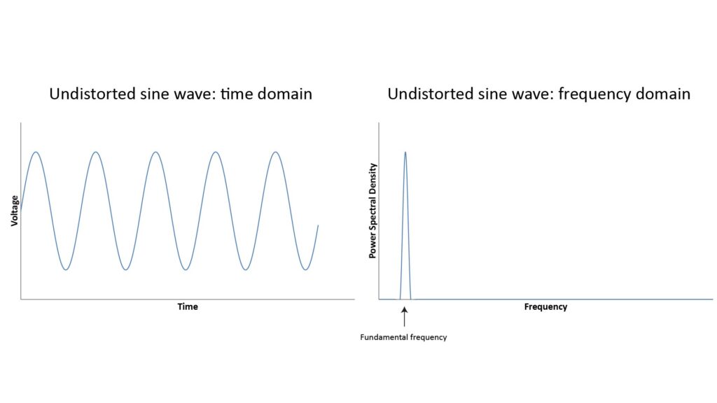
Let’s assume that the sound reaching the microphone is a pure tone. If the microphone has a perfectly linear response, then the output voltage should be a perfect sine wave, so that the Power-Spectral Density (PSD) of the output voltage will have a single spike at the tone’s frequency, as shown in the following figure:

But if there is any non-linearity in the microphone’s response, then the output won’t be a perfect sine wave; for example, it could have a flattened shape or there might be discontinuities at the zero-crossing points. And if the shape isn’t a perfect sine wave, then we know from Fourier analysis that its PSD cannot be a single spike at the tone’s fundamental frequency (since a single spike represents a perfect sine wave); instead, there must also be some signal power at other frequencies. For example, the following chart shows a clipped sine wave (as might occur when a microphone’s SPL-handling capacity is exceeded), along with the associated PSD:

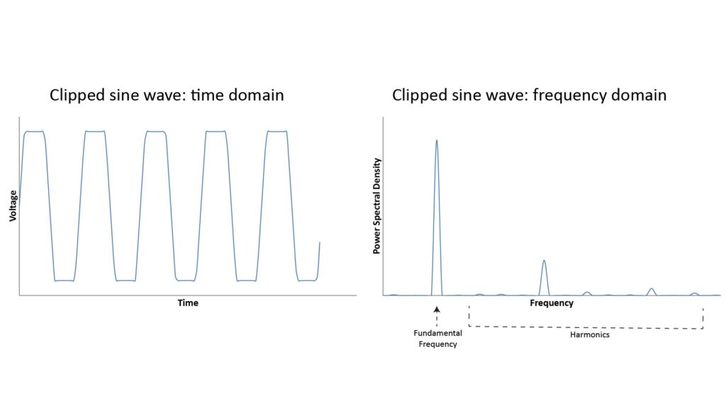
The spikes in the frequency domain other than the fundamental frequency are called harmonics; they appear at multiples of the fundamental frequency, and their magnitude and location will depend on the type and degree of non-linearity in the microphone’s response. But we know that if the original sound is a pure tone, then any power in the mic’s output at a frequency other than the tone’s fundamental frequency must be due to distortion.

And that’s the basis of THD: it represents the ratio of the power contained in all the harmonics to the power at the fundamental frequency, when the microphone is receiving a pure tone at 1 kHz.

How much THD is too much?

There’s a lot of debate in audiophile circles about how much THD is audible and how low a THD is necessary for “high fidelity”. I’m not going to get into that debate here, but I’ll just observe that a THD of ≤ 1% is generally considered good for a microphone, and even 3% may not be audible in speech or music.

How high SPLs cause THD

The THD at relatively high SPL levels is caused by the fact that a microphone’s diaphragm is capable of only a finite amount of travel, and at SPLs approaching the max distortion-free SPL, the diaphragm starts to bump-up against that travel limit. At this point, the microphone output is no longer linear with the sound pressure (or volume velocity, in the case of a pressure-gradient microphone), and this non-linearity begins to cause distortion. The distortion is still virtually inaudible at this level (hence the term “maximum distortion-free SPL”), but if the SPL increases still further, the distortion also increases until audible clipping eventually occurs, rendering the output useless for most purposes.

Relationship between maximum distortion-free SPL, microphone size, and sensitivity

Because the increase in THD at high SPLs is due to non-linearities in the diaphragm’s response to incident sound, the larger the diaphragm’s linear range of motion, the greater the maximum distortion-free SPL. Larger diaphragms have a greater linear range of motion than smaller diaphragms, so all other things being equal, a large-diameter microphone will tend to have a higher max distortion-free SPL than a small-diameter microphone.

However, all other things are not always equal. If the diaphragm’s movement is relatively stiff, it won’t move as much with a given SPL, and will therefore have a relatively high max distortion-free SPL. But that stiffness also reduces its sensitivity; this generally isn’t a significant issue, but it does increase the required downstream gain (more on that later). So a smaller microphone can have a higher max distortion-free SPL than a larger mic, but only if it’s much less sensitive.

Typical maximum distortion-free SPL specs

Not all manufacturers share my belief that maximum SPL is one of the key microphone specs; many microphone element datasheets don’t even specify it.

For example, two of the largest electronics distributors—Digi-Key and Mouser—don’t include a maximum SPL, THD, or AOP spec in their search filters for microphone elements; you have to open each microphone’s datasheet and find that spec yourself (if it exists).

However, maximum SPL (or a related spec) is usually quoted for high-quality microphone elements, and is always provided for high-quality complete microphones.

A survey of microphone max SPL specifications is beyond the scope of this post, but the following table gives an idea of typical specs, and how they’re presented, for various types of microphone:

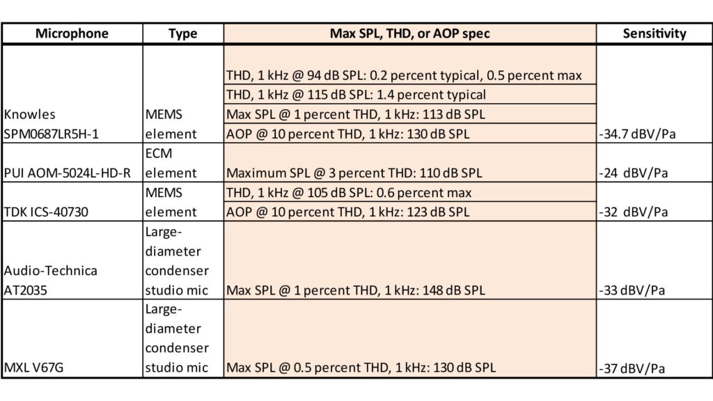
In addition to the various ways in which the specs related to maximum SPL and THD are presented, Table 1 suggests two facts about microphone max SPL:

• Small-diameter MEMS and ECM elements have lower maximum SPLs than large-diameter condensers, which are generally much more expensive.
• There is an inverse correlation between sensitivity and max SPL; note that the mic with the lowest max SPL (the AOM) has the highest sensitivity. Of course this is an extremely small sample size, but the inverse relationship between sensitivity and max SPL is, indeed, generally valid for microphones of the same size and type.

How high a max SPL do we really need?

The maximum distortion-free SPL is important for obvious reasons when extremely loud sounds must be recorded. But even sounds that are nominally quiet can exhibit momentary SPL spikes that can exceed the capacity of a microphone with a low maximum SPL rating—especially when the microphone is located very close to the source.

The following figure shows the SPL at the microphone versus the source-to-microphone distance for various loud sounds:

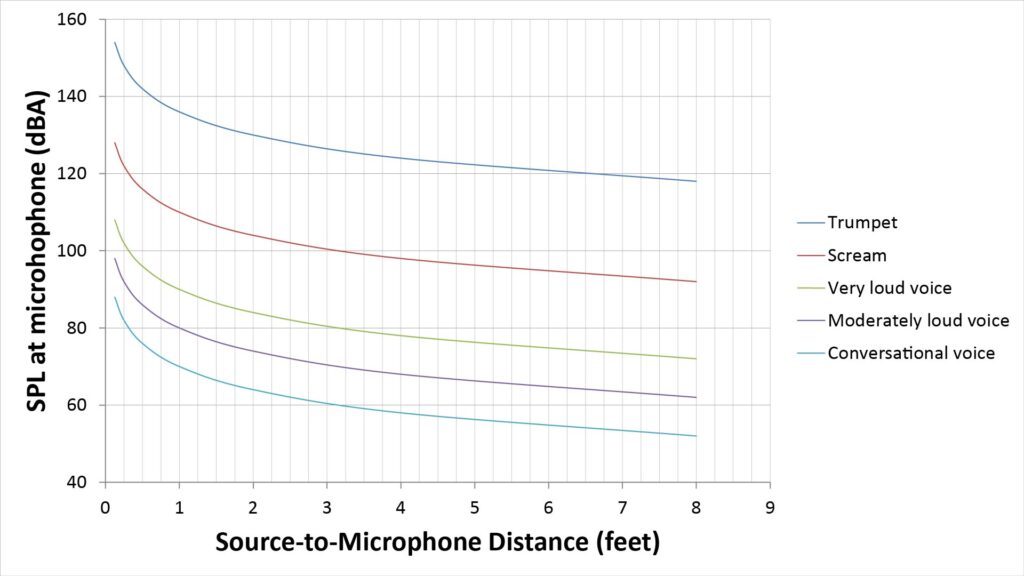
We can see that a microphone used for picking-up conversational voice might see a maximum SPL of about 90 dB SPL, whereas a microphone used for live vocals or musical instruments might see as much as 130 dB SPL or even more. We can also see that the SPL varies by about 20 dB between a 1-foot source-to-mic distance (typical for a studio mic) and a 3-inch source-to-mic distance (typical for a mic held close to the mouth or a headset mic).

One of the most significant conclusions we can draw from all this is that the relatively limited SPL capacity of small-diameter microphone elements won’t be an issue for many applications; a relatively expensive large-diameter element is absolutely necessary only for close-miking loud sounds.

Effective Input Noise (EIN), aka self-noise

The output of any microphone, whether powered (active) or unpowered (passive), will always contain some electrical noise produced in the microphone itself. This noise can be measured by putting the microphone in a soundproof chamber and measuring the output power over the audio bandwidth (20 Hz to 20 kHz), typically with A-weighting applied to reflect the nominal frequency response of the human ear.

The level of this electrical noise is usually expressed as the SPL of a fictitious acoustic noise at the microphone diaphragm that would result in the same electrical noise at the output if the microphone were noise-free. For example, the output of a microphone with a self-noise of 14 dBA (like the Audio-Technica AT4021), when placed in a sound-proof chamber, would be the same as that of a fictitious noise-free microphone operating in an ambient noise level of 14 dBA. The concept of EIN is illustrated in the following figure:

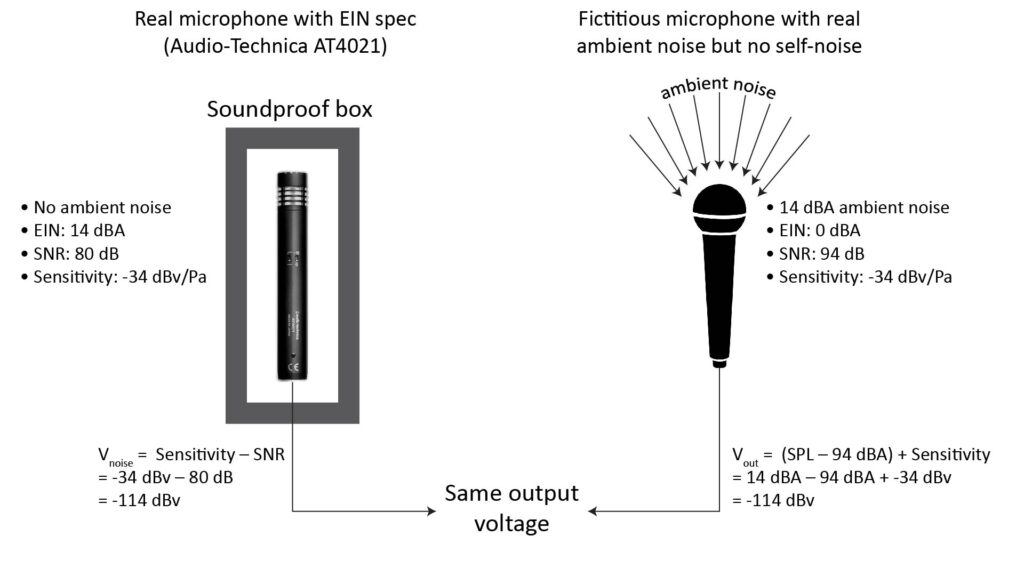
Hence, the self-noise expressed in dBA is more accurately described as the Equivalent Input Noise (EIN).

EIN versus Signal-to-Noise Ratio (SNR)

Microphone self-noise is also sometimes implicitly specified via the Signal-to-Noise Ratio (SNR) spec, wherein the “signal” is always a standard reference sound pressure level (specifically 1 Pascal, or 94 dBA).

Because the signal level is always the same, the only real information conveyed by the SNR spec is the microphone noise. In fact, the EIN and the SNR differ only by the 94 dB SPL constant:

• EIN (in dBA) = 94 dBA – SNR, or
• SNR = 94 dBA – EIN

Why doesn’t a microphone’s SNR depend directly on its sensitivity?

Since the acronym SNR has an “S” for “signal” in it, it might seem that SNR would directly depend on the microphone sensitivity. It doesn’t, and that’s because both the Signal and the Noise in the SNR spec are in terms of SPL levels at the microphone input.

On the other hand, microphone sensitivity refers to the microphone’s output in millivolts (mV) for the standard reference tone with a sound pressure of 1 Pascal (94 dB SPL) at 1 kHz. So, SNR and sensitivity are independent specs. However, the sensitivity does determine the noise voltage for a given EIN (or SNR), as follows:

• v_noise = Sensitivity – SNR, where v_noise is the noise voltage in dBV, sensitivity is in dBV, and SNR is in dB.

Also, I have seen evidence of a loose correlation between EIN and sensitivity, with high-sensitivity microphones tending to have higher EINs than low-sensitivity microphones (although this is by no means a firm rule).

What determines microphone EIN

All electrical devices at temperatures above absolute zero produce thermal noise (also called Johnson-Nyquist noise), which is the only significant source of noise in passive (un-powered) microphones. The amount of thermal noise depends on the temperature and the resistance across which the noise is measured, and the RMS noise voltage further depends on the bandwidth:

• v_n = Sqrt(4k_BTRB), where v_n is the RMS noise voltage, k_B is Boltzmann’s constant (1.38×10^-23 Joules per Kelvin), T is the temperature in Kelvins, R is the resistance in ohms, and B is the bandwidth in Hz.

For low-impedance un-powered microphones (such as dynamic mics), the noise voltage over audio bandwidths is negligible because it will almost certainly be below the noise due to any actual ambient noise reaching the microphone diaphragm.

On the other hand, powered microphones (such as condenser microphones) produce other types of noise in addition to thermal noise. The element itself (whether an externally-polarized condenser or an internally-polarized Electret condenser) produces some noise, as does the impedance buffer necessary to extract a useful signal from the extremely high impedance of the condenser. The buffer is usually a Junction Field-Effect Transistor (JFET) but can also be a vacuum tube.

The two types of significant noise (other than thermal noise) produced in powered microphones are shot noise and I/f noise (sometimes called flicker noise). These are the dominant noise sources in powered microphones, being much larger than the thermal noise. The exact mechanisms that give rise to these types of noise is beyond the scope of this discussion (and, in the case of the condenser element itself, not well-understood), but three facts are clear:

• Unlike the situation with dynamic microphones, the EIN of powered microphones can easily be high enough to be audible—and is therefore an important consideration in microphone selection.
• Condenser microphone EIN tends to vary inversely with microphone element size: all other things being equal, larger mics usually have lower EIN than smaller mics.
• As previously mentioned, there seems to be some correlation between EIN and sensitivity, with more sensitive microphones tending to have higher EIN…although there are plenty of exceptions to this.

Typical microphone EINs

Microphones can be divided into four broad classes based on EIN/SNR, as shown in the accompanying table:

EIN	Typical microphone type	Comments
<10 dBA	Large-diameter condenser, dynamic, small-diameter array microphone	Extremely low self-noise; virtually inaudible even in the quietest environments
≥10, <20 dBA	Large-diameter condenser, high-quality small-diameter condenser	Low self-noise; inaudible unless ambient noise is extremely low (such as in a soundproof recording booth); suitable for all but the most demanding applications
≥20, <30 dBA	Small-diameter condenser, piezoelectric MEMS	Medium self-noise; marginally audible in quiet environments (such as in a home recording studio); highest acceptable EIN for general-purpose use
≥30 dBA	Small-diameter condenser, piezoelectric MEMS	High self-noise; audible except in high ambient noise; not recommended because lower EINs are possible without excessive cost or compromise in other specs

Why microphone EIN is important

The importance of EIN is pretty obvious, and the fact that it’s expressed in dB-SPL (referred to a fictitious acoustic noise at the microphone diaphragm) makes its significance easy to understand: the EIN will be audible in the microphone’s output if it approaches the actual acoustic noise level.

This means that, for good performance, we need the EIN to be comfortably below the minimum expected acoustic noise level (I use a margin of at least 6 dB, but some people recommend 10 or even 15 dB). Unless you’re using a microphone in an acoustically treated (or at least a very quiet) room, this is pretty easy to achieve even with a reasonably-priced microphone.

The following table lists ambient noise levels for typical environments, along with the associated maximum EINs based on a 6 dB margin:

Environment	Typical Ambient Noise Level	Maximum EIN (assuming 6 dB margin with ambient noise)
Restaurant	70 dBA	64 dBA
Living room	60 dBA	54 dBA
Library	50 dBA	44 dBA
Private office	40 dBA	34 dBA
Home recording studio	30 dBA	24 dBA
Professional recording studio	20 dBA	14 dBA

Polar response

A microphone’s polar response is its sensitivity to sound as a function of the sound’s angle of arrival. Polar response is often specified via a polar pattern, which is a plot showing the relative response as a function of angle in a given plane. Here’s an example of a polar pattern (this one is for the Audio-Technica AT4021):

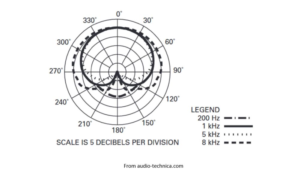
The polar pattern shown above is, like most polar patterns, two-dimensional: it shows the polar response in just a single plane, whereas an actual polar response is always three-dimensional. However, virtually all polar responses are also axisymmetric, meaning that they’re the same in two orthogonal planes (such as horizontal and vertical). That’s why only one polar pattern is usually given.

Directional polar patterns are always frequency-dependent

As shown in Figure 6, the AT4021 is more sensitive at zero degrees than at 180 degrees; it has a directional polar pattern (specifically a cardioid pattern, which we’ll discuss shortly), and it varies with frequency: the higher the frequency, the more directional the pattern.

There are five facts about the frequency-dependence of directional polar patterns to keep in mind:

• A directional polar pattern is meaningless unless it’s associated with a frequency.
• Because a directional polar pattern gets less directional with decreasing frequency, it becomes effectively isotropic (non-directional) at some point. You can see this trend in Figure 6: at 200 Hz, the AT4021 is starting to respond to sound from 180 degrees, and if the manufacturer had shown the response at 20 Hz, the pattern would start to look even more isotropic. The lowest frequency at which a microphone provides useful directivity depends on its design.
• While all directional polar patterns become increasingly directional with increasing frequency, there is a frequency above which every directional pattern falls apart. Specifically, the pattern starts to develop “fingers” (called lobes) at directions other than zero degrees, spoiling the directivity; this phenomenon is called spatial alaising. Again, this maximum usable frequency depends on the microphone design. A microphone manufacturer will rarely specify polar patterns above the aliaising frequency.
• If a polar pattern is specified at just a single frequency, it’s usually a frequency just below the aliasing frequency; that’s when the pattern is most directional and looks the best.
• There is a trade-off between the lowest frequency at which a microphone is effectively directional, and the highest frequency at which the pattern remains intact. In other words, all practical directional microphones have a finite bandwidth over which they provide useful directivity.

Polar response specifications

There are four commonly-used microphone specs related to the polar pattern, any one of which might be most relevant in a given application:

• Polar pattern shape
• Beamwidth
• Directivity and Directivity Index
• Distance Factor

Polar pattern shape

An infinite number of polar pattern shapes are possible depending on the microphone design. It’s useful to divide the possible patterns into two categories:

• The canonical or standard polar patterns. These are the most common directional patterns; they’re the five most useful patterns possible with a single microphone capsule that isn’t augmented with an acoustic device like a reflector or interference tube.
• High-directivity polar patterns. These require a specialized microphone design using multiple microphone elements (called an array microphone) or an acoustic directivity-enhancing device.

The following figure shows the five standard patterns along with a typical high-directivity pattern, for six hypothetical microphones at 10 kHz:

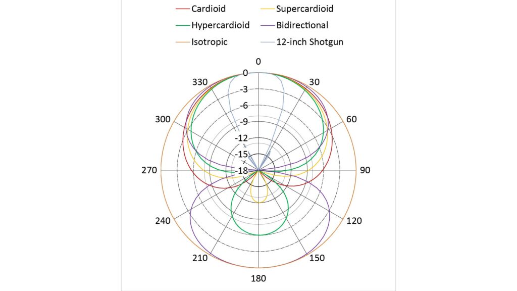
I calculated the bidirectional and cardioid-family polar patterns of Figure 7 assuming a spatial aliasing frequency of just above 10 kHz. In other words, the patterns of Figure 7 represent the most directional patterns possible with a bidirectional or cardioid-family microphone. In fact, all bidirectional or cardioid-family polar patterns presented without a frequency label represents the same thing: the pattern at the highest frequency before aliasing occurs.

For the shotgun microphone, on the other hand, a much more directional pattern would be possible by using a longer interference tube, and of course the pattern would be more directional at a higher frequency.

By the way, if you’re interested in how I calculated the patterns of Figure 7, check out the following:

• Bidirectional and cardioid-family polar responses are obtained using a pressure-gradient microphone element, and such elements work in exactly the same way as two-element differential microphone arrays. I show how to calculate the polar response of such microphones in my post on how array microphones work.
• I describe a model for how to calculate the polar response of a shotgun microphone in my post on how shotgun microphones work.

Beamwidth

The beamwidth is a measure of the sharpness of the polar response. It’s the angular width over which the microphone’s sensitivity is within a certain fraction of the peak sensitivity; this fraction is typically one-half (or, in dB, -3 dB). Such a beamwidth is referred to as the -3 dB beamwidth.

If the polar pattern has more than one dip in the response (which is called a null), then a beamwidth spec known as the null-to-null beamwidth is sometimes specified instead of the -3 dB beamwidth.

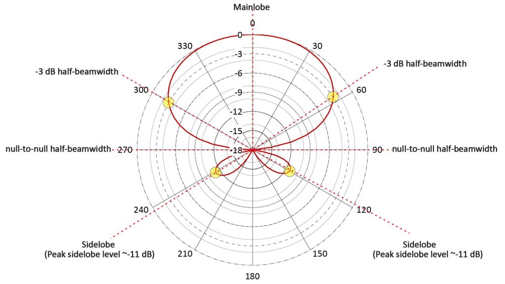
The beamwidth is usually a useful spec only for specialized microphones that have a very sharp polar response (such as parabolic microphones); it gives an idea of how accurately the microphone must be pointed at the source.

Directivity and Directivity Index

One of the key benefits of a microphone with a non-isotropic polar response is the ability to preferentially pick up sound from a desired direction while ignoring sounds from other directions. This ability can be quantified via a metric known as Directivity (D), which is defined as the ratio of the peak sensitivity to the sensitivity averaged over all directions. Directivity is most commonly specified in dB as the Directivity Index (DI).

One of the benefits of a high DI is that it suppresses ambient noise, which is often the greatest impediment to capturing high-quality sound. If the ambient noise is isotropic (arriving with equal strength from all directions), which is usually the case, then the DI represents the dB reduction in the ambient noise level provided by the microphone.

Distance Factor (DF)

In addition to suppressing high levels of ambient noise, a high DI is also useful in low-ambient-noise conditions to extend the useful pick-up range of the microphone. This is because the Sound Pressure Level (SPL) of the desired sound drops with increasing distance from the source, so that even a low level of ambient noise can interfere with it. By reducing the ambient noise, a high DI allows the mic to be moved further from the source while maintaining the same sound quality. See my post on how well parabolic and othe long-range directional microphones work for much more detail on the challenges of picking-up sound at long range.

The increased pick-up range enabled by directivity is quantified as the Distance Factor (DF), which is the increase in range at which the drop in the desired sound’s SPL is exactly offset by the reduction in ambient noise. For example, a DF of two means that the distance can be doubled while maintaining the same margin over the ambient noise.

The DF can be estimated from the DI as follows:

• DF = 10^(DI/20), where DF is the distance factor (unitless) and DI is the Directivity Index in dB.

Directivity and Distance Factor aren’t necessarily frequency-dependent

While the shape of a directional polar pattern always varies with frequency, its Directivity (and therefore the Distance Factor) don’t necessarily vary with frequency.

In particular, the D and DI provided by the bidirectional and cardioid-family polar patterns of Figure 7 are constant for all frequencies up until the spatial aliasing frequency. This is because, as the beamwidth changes with frequency, the width of the null changes in the same way. For example, as the beamwidth gets broader with decreasing frequency (which would tend to reduce D), the null at 180 degrees also gets broader (which tends to increase the directivity). These offsetting factors result in a constant D.

This isn’t the case, however, for most polar patterns that have a directivity greater than 6 dB.

In fact, except in the case of esoteric microphone designs, the directivity of microphones with high directivity (a DI greater than 6 dB) is always frequency-dependent: it increases with frequency. See this section of my post on directional long-range microphones for some examples of directivity-versus-frequency curves for typical highly-directional microphones.

There are two practical implications of this:

• DIs at high frequencies are relatively easy to achieve, but achieving a DI of greater than 6 dB at low frequencies requires a physically large device—often too large to be practical.
• Because the DI is frequency-dependent, so are the ambient noise suppression and Distance Factor (DF). That complicates performance predictions for high-directivity microphones; I’ll discuss that in more detail in an upcoming post on how to predict microphone performance.

Polar response characteristics for typical microphone configurations

The following table lists the DIs and beamwidths for all five standard polar responses, as well those for two types of high-directivity microphone (shotgun and parabolic):

Polar pattern shape or microphone type	-3 dB Beamwidth (degrees)	Directivity	Directivity Index (DI)	Distance Factor (DF)	Notes
Isotropic	360 degrees	1.0	0 dB	1.0	Best for short ranges, when ambient noise isn’t an issue, or when mic orientation to source can’t be controlled. Usually offers best specs other than polar response
Bidirectional (Figure-8)	90 degrees at max usable frequency	3.0	4.7 dB	1.7	Best for suppressing sound from the sides; essential for some multi-channel recording set-ups
Cardioid	131 degrees at max usable frequency	3.0	4.8 dB	1.7	Best for suppressing sounds from the rear (e.g. to minimize risk of feedback when recording live performances)
Super-cardioid	115 degrees at max usable frequency	3.7	5.7 dB	1.9	Not as effective as the cardioid for suppressing sounds from the rear, but offers the highest front-to-back ratio of all the standard responses
Hyper-cardioid	105 degrees at max usable frequency	4.0	6.0 dB	2.0	Even less effective than the supercardioid at suppressing sounds from the rear, but offers the highest DI of all the standard responses
Pencil beam (typical 12-inch shotgun microphone) at 2 kHz	70 degrees at 2 kHz	10.0 at 2 kHz	10 dB at 2 kHz	3.2	Shotgun microphone directivity increases with frequency at 3 dB per octave. See how shotgun microphones work for more detail.
Pencil beam (typical 22-inch parabolic microphone) at 2 kHz	20 degrees at 2 kHz	50.0 at 2 kHz	17 dB at 2 kHz	7.1	Parabolic microphone directivity increases with frequency at 6 dB per octave. See how parabolic microphones work for more detail.

Why is microphone polar response important?

As already mentioned, microphone polar response (and specifically as high a DI as possible) is the key determinant of microphone performance in the presence of isotropic ambient noise, or when attempting to pick-up sound at long ranges.

There are also two other applications in which polar response is often the most important performance microphone attribute:

• In the presence of anisotropic ambient noise. While ambient noise is most often isotropic, there are situations in which much of the noise comes from a single general direction. A classic example of such an anisotropic noise situation is miking a singer in an amplified live performance; the microphone needs to suppress the sound coming from the speakers in order to avoid feedback. Suppressing anisotropic noise requires a polar response that has negligible sensitivity in the direction of the offending sound (referred to as a null in the polar pattern). Achieving a deep null is much easier than achieving a high DI, and an ordinary cardioid pattern is excellent in this regard (a noise suppression of 20 dB or more is possible at 180 degrees off-axis).
• Capturing sound for multi-channel imaging formats. Multi-channel formats such as stereo, surround-sound, and Ambisonics require unidirectional or bidirectional microphones to achieve the desired imaging and/or ambience. As with anisotropic ambient noise, this application doesn’t require a high DI, and one of the standard polar patterns (typically a bidirectional or cardioid pattern) is usually optimum.

There is also another microphone use-case in which polar response is indirectly important. This is to achieve the proximity effect, which is the bass boost that occurs when a microphone with a non-isotropic response is located very close to a sound source. Some singers and podcasters prize the bass-heavy “FM DJ” sound caused by the proximity effect, and it can be effectively turned on and off as desired by moving closer to and further from the mic. The proximity effect isn’t directly related to a microphone’s polar response, but there is an indirect relationship because any microphone that doesn’t have an isotropic response uses a form of pressure-gradient microphone, and all pressure-gradient microphones exhibit the proximity effect to at least some extent. BTW, if you’re curious about the physics behind the proximity effect, check out this explanation in my post on how array microphones work.

Effective bandwidth

“Effective bandwidth” is my own term for a particular way of characterizing frequency response. I’ll briefly go over frequency response before addressing what I mean by effective bandwidth.

A microphone’s frequency response reflects its sensitivity to sound (in the direction of peak sensitivity) as a function of the sound’s frequency. As with polar response, frequency response can be specified graphically (via a frequency response curve) or via metrics such as bandwidth.

As with angular beamwidth, bandwidth refers to the range of frequencies over which the sensitivity is within a certain fraction of the peak. The -3 dB bandwidth is the one most frequently specified, but the bandwidth over a larger range (such as -12 dB) can also be specified.

The following figure illustrates these concepts:

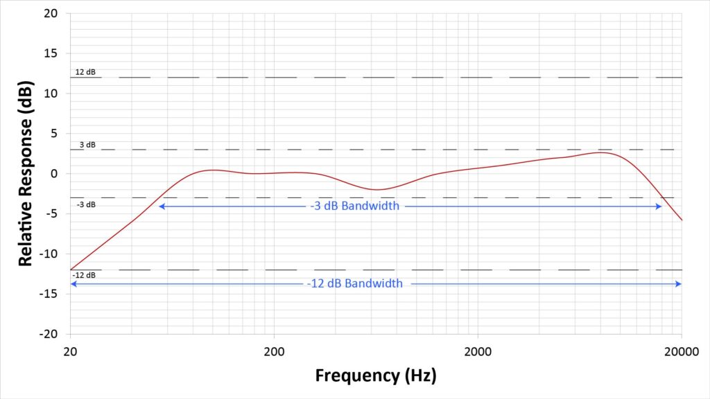
When most people look at an audio device’s spec sheet, they’re looking for a reasonably flat frequency response across the entire audio bandwidth of 20 Hz to 20 kHz. In electronics, “reasonably flat” is generally considered to be “within 3 dB”, so a -3 dB bandwidth of 20 Hz to 20 kHz is the gold-standard for microphone frequency response.

A flat frequency response isn’t always necessary or even desirable

However, while a reasonably flat response from 20 Hz to 20 kHz is nice, it usually isn’t necessary. That’s because a microphone’s output can be—and often is—equalized by applying a frequency-dependent gain or attenuation to achieve a desired frequency response. Further, the desired frequency response depends on how the signal will be used (and on the tastes of the person doing the equalization), and usually isn’t perfectly flat from 20 Hz to 20 kHz. By the way, I have a detailed post on microphone equalization in the works.

Another issue with a flat frequency response is that achieving a broad, flat response often necessitates compromises in other aspects of microphone performance. This is especially true with microphones that have an anisotropic polar response (like cardioid-type studio mics).

So, while it might be tempting to specify a -3 dB bandwidth of 20 Hz to 20 kHz, it isn’t necessary for good performance—and relaxing the bandwidth requirement in favor of downstream equalization can actually result in better overall signal quality.

Limits of microphone equalization

However, there are a few downsides to equalization (aside from the need for a device or app to perform it): increased noise, the potential for audible artifacts due to the equalizer’s phase response, and the potential complexity of the required equalizer.

Increased noise

Equalization involves either attenuating the frequencies that are over-emphasized in the raw frequency response, or else amplifying the frequencies that are under-emphasized—and both add noise to the output signal in different ways:

• Attenuating the over-emphasized frequencies reduces the effective sensitivity of the microphone, requiring greater downstream gain to maintain the desired signal level. All audio gain stages add some noise to the signal, and the amount of added noise increases with the gain.
• Amplifying the under-emphasized frequencies also amplifies the microphone’s self-noise along with the signal.

Also, in both cases the equalization itself (whether via attenuation or gain) adds a bit of noise.

The increase in noise depends on the design of the equalizer and the following gain stage(s), and it’s frequency-dependent (because the equalization is, by definition, frequency-dependent). It’s not too hard to get an estimate of the increase in noise caused by equalization, but it’s beyond the scope of this post.

Potential for audible artifacts due to phase response

Any device that has a non-flat frequency response (like an equalizer) always has a non-flat phase response, and some people believe that an equalizer’s non-flat phase response can induce audible artifacts in the equalized signal. I myself have seen no evidence of this phenomenon when equalizing smooth frequency roll-offs of up to 12 dB per octave, but steeper roll-offs seem difficult to equalize without audible artifacts. Another factor is that steep roll-offs require more gain for the same bandwidth, which exacerbates the noise gain mentioned above.

Potential Equalizer complexity

Equalizing one end (either the low-end or high-end) of a gradually drooping frequency response can be done with a relatively simple equalizer. However, equalizing a ragged frequency response with many peaks and valleys requires multiple parametric filters that, in addition to increasing the potential for audible artifacts, also requires a relatively complicated equalizer.

What can and cannot be equalized

There are definitely limits to microphone equalization for the reasons mentioned above. There are no hard-and-fast rules, but my experience has been that a single frequency-response droop of up to 12 dB (and sometimes as much as 24 dB) with a slope of up to 12 dB per octave, can be equalized easily and without audible artifacts. The following types of frequency-response aberrations fall into this category:

• A 6 dB-per-octave high-frequency roll-off due to diaphragm mass. This allows the high-frequency response of a pressure-microphone to be extended by one or two octaves.
• The 6-dB-per-octave low-frequency roll-off of a parabolic microphone or a differential array microphone. However, parabolic mics present another issue for low-frequency equalization (beyond the noise and complexity factors mentioned above): the ambient-noise rejection also falls off at 6 dB per octave. So ambient noise, rather than electronic noise, can limit the achievable bandwidth extension from equalization. Still, one or two octaves of low-frequency extension are generally possible; see how parabolic microphones work for more detail.
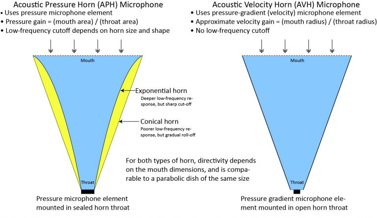
• The low-frequency roll-off of conical horn microphones (conical horns have a more gradual low-frequency roll-off than exponential horns; see how horn microphones work for more detail).

On the other hand, steeper droops or multiple dips and valleys are difficult to practically equalize. One example is the high-frequency aliasing that can occur in array microphones (which I discuss in detail in how array microphones work).

Effective bandwidth is the bandwidth over which the response can be effectively equalized

With that background, we can now discuss the concept of effective bandwidth: it’s the range of frequencies over which the microphone’s output can be equalized without adversely affecting the quality of the output signal.

So, referring again to Figure 9, if we can safely apply 12 dB of equalization to the signal, then the effective bandwidth would be the -12 dB bandwidth, rather than the narrower -3 dB bandwidth that’s typically specified—assuming that roll-off(s) to be equalized aren’t too steep.

As noted above, if reasonably quiet electronics are used, up to ~24 dB of equalization is possible without increasing the overall audible noise level at the output (where “overall” includes any actual acoustic ambient noise reaching microphone diaphragm). I’ll address this in much more detail in an upcoming post.

Therefore, a microphone’s effective bandwidth is more like the -24 dB bandwidth than the -3 dB bandwidth, assuming a smooth roll-off(s) no greater than ~12 dB per octave.

But how do we determine the required effective bandwidth?

Required effective bandwidth

From a bandwidth-requirements standpoint, we can divide most microphone applications into two categories: those intended to capture only voice, and those intended to capture music as well as voice (there are also other more esoteric applications which we’ll discuss later):

• When capturing music, we care about fidelity: we want the captured signal to represent the music as accurately as possible.
• We might also be interested in fidelity when capturing voice. However, in many voice-capture applications, what we really care about is intelligibility: how well the voice can be understood. And, as we’ll see, intelligibility takes significantly less bandwidth than fidelity.

When fidelity is important

Regardless of the type of sound being captured, it’s safe to say that maximum fidelity requires a microphone bandwidth that spans the full audio range, or about 20 Hz to 20 kHz.

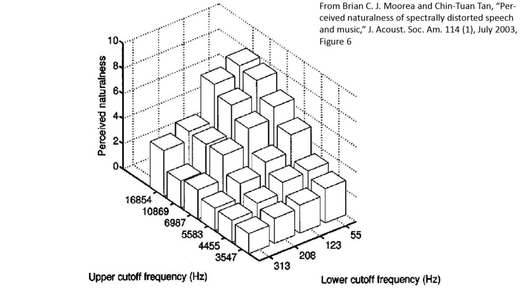
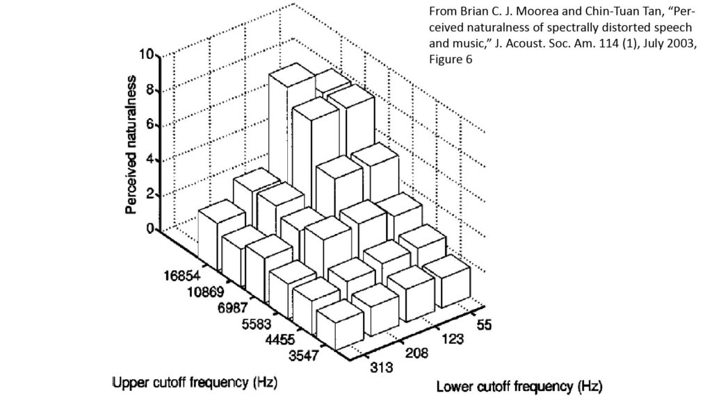
But what if some fidelity can be sacrificed? In other words, how does fidelity vary with bandwidth? That’s not an easy question to answer because fidelity is subjective. One interesting study that sheds some light on this topic was undertaken by Moore and Tan [1], who polled various listeners to determine the perceived naturalness of band-limited music and speech (they also investigated the effect of other forms of distortion, like spectral ripples and tilts).

The study methodology was too complex to describe in detail here (the paper is available online for free if you’re interested in the details; see the reference citation at the bottom of this post), so I’m going to hit just the high points:

• The study asked ten subjects without hearing impairment (ranging in age from 15 to 31) to rate sample sounds (both music and speech) on a ten-point naturalness scale, where 10 represented “very natural—uncolored” and 0 represented “very unnatural—highly colored”.
• To help calibrate the responses, the subjects were first presented with undistorted, full-bandwidth samples as examples of sounds that merited a score of 10. This “full” bandwidth was 55 Hz to 16,854 Hz.
• They were then asked to rate the naturalness of sample sounds that had been band-limited to each of 24 different bandwidths. For each bandwidth, the upper edge was defined by one of six different low-pass cutoff frequencies and the lower edge by one of four different high-pass cutoff frequencies. In the following discussion, I’m going to refer to each bandwidth as “A/B Hz”, where A is the lower edge and B is the upper edge.
• The widest sample bandwidth was 55/16,854 Hz, while the narrowest was 313/3,547 Hz. For reference, the later is almost exactly the bandwidth of traditional telephony (versus the 50/7,000 Hz bandwidth of HD telephony now offered in most major markets).

Figures 10 and 11 summarize the results of the bandwidth portion of the study:

We can make a few observations about the data before we attempt to translate it into bandwidth requirements:

• Surprisingly (at least to me), the naturalness of music decreases more gradually than the naturalness of speech as the bandwidth is reduced below full bandwidth (note the relatively large decrease for speech with bandwidths less than 123/10,869 Hz).
• A bandwidth that extends down to ~100 Hz is very important for high fidelity (especially for speech); note the steep drop-off in naturalness when the upper edge of the bandwidth is greater than 10,869 Hz but the lower edge increases above 123 Hz.
• The study authors observe that a poor LF response sharply reduces the benefits of a good HF response, and that a poor HF response sharply reduces the benefits of a good LF response. However, just as significant to me is the fact that there is still at least some benefit from a good HF response when there is a poor LF response, and vice-versa. This is especially true for music, as shown in Figure 10:
  • When the LF response is limited to 313 Hz, the naturalness is noticeably greater for an HF response of 16,854 Hz than for an HF response of 10,869 Hz.
  • When the HF response is limited to 3,547 Hz, the naturalness is noticeably greater for an LF response of 55 Hz than for an LF response of 313 Hz.

So, what does this data tell us about bandwidth requirements? It shows that fidelity (as proxied by the naturalness scores) decreases as the bandwidth is reduced, which we already knew (or at least expected). But what’s useful about the data is that it seems to suggest several distinct fidelity regimes that we can use as a basis for bandwidth requirements. By eyeballing the chart (and corroborated by my own experience), I arrived at the following bandwidth requirements for five distinct fidelity regimes:

Fidelity regime	Lower edge of bandwidth	Upper edge of bandwidth
Poor: equivalent to traditional telephony	≤300 Hz	≥3,500 Hz
Marginal: noticeably better than traditional telephony, but still not good	≤200 Hz	≥5,600 Hz (speech) or 7,000 Hz (music)
Good: probably adequate for general-purpose use	≤120 Hz	≥11,000 Hz
Very good: adequate for almost all purposes	≤60 Hz	≥17,000 Hz
Excellent: when the highest possible fidelity is needed	≤20 Hz	≥20 kHz

When intelligibility, but not necessarily fidelity, is important

Some voice applications (such as for surveillance and communications) don’t require high fidelity, but do require high intelligibility: the voice doesn’t have to sound natural, but it does have to be understandable. As you might expect, the importance of various frequencies for vocal intelligibility has been studied extensively in the field of audiology.

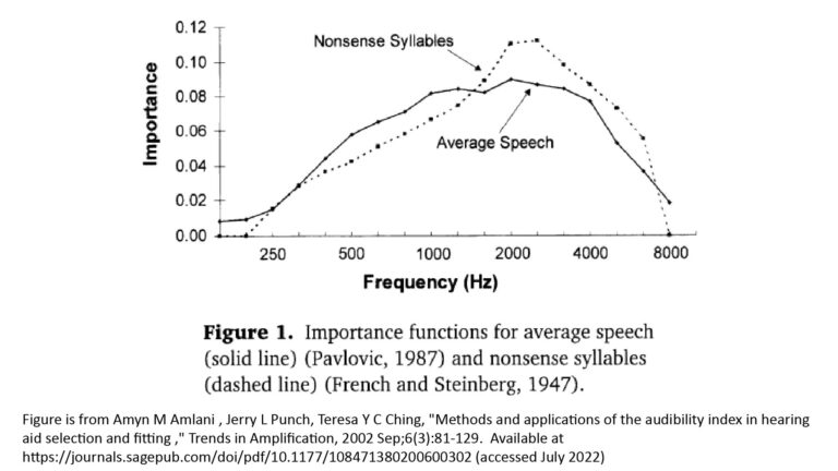
This has typically been done by having volunteers attempt to identify vocal sounds (sometimes continuous speech, sometimes individual words, and sometimes nonsense syllables) that have been band-limited (filtered) in various ways. This enables the importance of each frequency to overall intelligibility to be characterized via a frequency importance function.

For example, the following figure plots the frequency-importance function obtained by Studebaker et al [2] for continuous discourse (speech). Note that while this data is quite dated (the study was published in 1987), it’s still valid enough for our purposes:

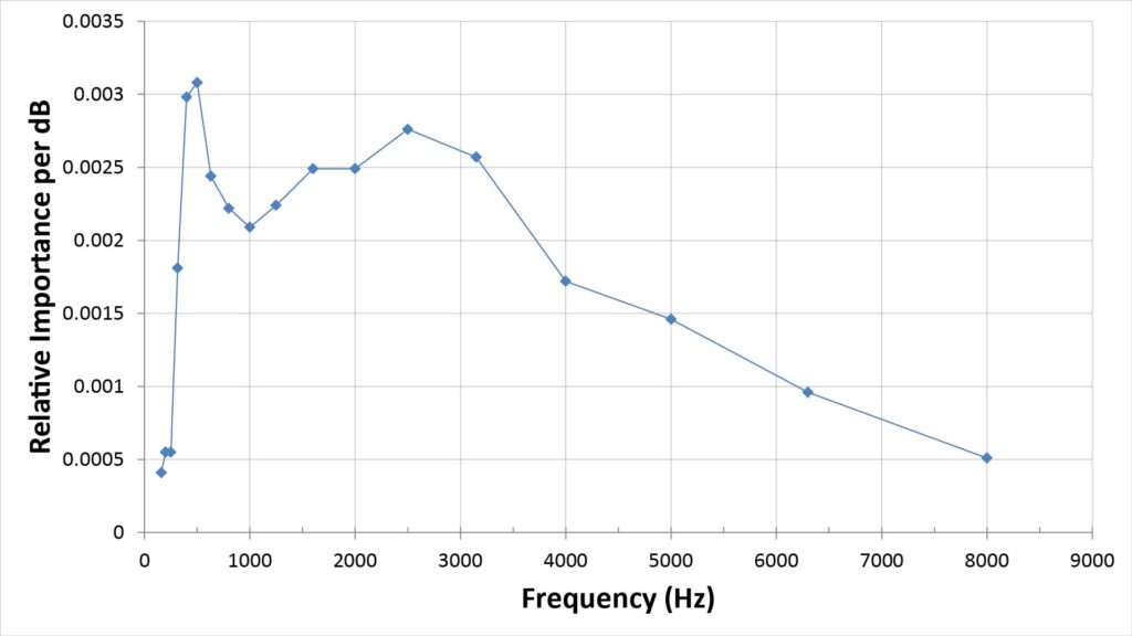
Note the stark differences between the frequency-importance function of Figure 12 and the speech naturalness scores of Figure 11:

• The frequency-importance function shows that frequencies below 500 Hz contribute little to intelligibility, and in fact the bulk of the intelligibility is due to frequencies above 1 kHz. On the other hand, the naturalness scores show that frequencies below 313 Hz contribute quite a bit to fidelity.
• The frequency importance function shows that frequencies above 3.5 kHz contribute relatively little to intelligibility, whereas the naturalness scores show huge contributions to fidelity from frequencies above 5,583 Hz.

We can draw a few conclusions from Figure 12:

• If we want high intelligibility but not necessarily high fidelity, then we need a bandwidth that goes at least as low as 400 Hz and at least as high as 6 kHz.
• If we need only marginal intelligibility (and if poor fidelity is acceptable), then a bandwidth of 1 kHz to 4 kHz may suffice. This is particularly relevant for long-range surveillance applications.

By the way, the bandwidth requirements for voice pick-up are discussed in more detail in this section of my post on long-range microphones.

Bandwidths for specialized applications

There are also a few specialized microphone applications in which the above guidelines don’t apply:

• Capturing wildlife sounds. Of course, the required bandwidth in this case depends on the type of wildlife to be captured. In general, the smaller the animal, the higher the frequency of the sounds it makes (see Fletcher [3] for a simple model that relates the center frequency of an animal’s vocalization to its body mass). Very few animals produce frequencies lower than 20 Hz, but many produce frequencies much higher than the human hearing limit of 20 kHz. The most familiar example of a microphone intended for wildlife applications is probably the parabolic microphone. As described in detail on my post on how parabolic microphones work, a parabolic mic’s gain and directivity increase with increasing frequency, so they’re ideal for capturing high-frequency wildlife sounds at long range.
• Capturing the sounds of geophysical phenomena (such as storms and earthquakes) or large machinery (such as diesel locomotives and power plants). These sounds include plenty of power below the 20 Hz lower limit of human hearing. Detecting such infrasonic frequencies isn’t difficult, but distinguishing the desired sound in the presence of low-frequency noise (such as due to wind gusts) can be a real challenge.
• Ultrasonic sensing, such as for motion-detection and distance-measurement applications. This typically requires a specialized sensor, although some inexpensive microphones and speakers can be used to sense sound below 40 kHz or so.

A less important (but still important) spec: microphone sensitivity

A microphone’s sensitivity is its output voltage per unit sound pressure level. Sensitivity is important but it doesn’t typically have as much impact on performance as other specifications.

How sensitivity is specified

A microphone’s rated sensitivity is its output voltage in response to a reference sound pressure of 1 Pascal (1 Pa) which is equal to 94 dBZ SPL) at 1 kHz. It’s expressed in dB_V/Pa (or sometimes, erroneously, as just “dB”) as:

• S = 20log(V_out), where S is the sensitivity in dB_V/Pa and V_out is the microphone output in Volts for a 1 kHz tone at a 94 dB SPL (equation 1)

Conversely, the microphone output voltage for a given sensitivity and SPL can be found as follows:

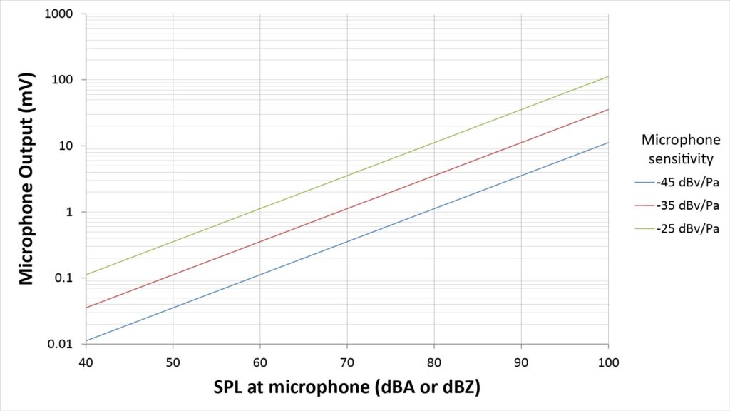
• V_out = 10^[(S+SPL-94)/20] Volts, where S is the rated sensitivity in dB_V/Pa and SPL is the sound-pressure level (equation 2)

So, a microphone with a sensitivity of -40 dB_V/Pa has an output of 10^(-50/20) V, or 3 mV, for an SPL of 94 dB. If the SPL increases by 6 dB to 100 dB SPL, then the output should also increase by 6 dB to 6 mV.

However, equation 2 only applies if the SPL is below the maximum SPL capacity of the microphone; otherwise, the output will be less than predicted by equation 2 as the microphone begins to clip.

Similarly, equation 2 only applies if the SPL is above the microphone’s self-noise; otherwise, the output will be determined by the microphone’s EIN, rather than the actual SPL…and it will be noise, rather than a useful signal.

The following figure shows microphone output, in mV (millivolts) as a function of SPL, for three different values of microphone sensitivity:

Why sensitivity is important

The main significance of microphone sensitivity is that it determines the required sensitivity or gain of the downstream device: microphones with low sensitivity need more downstream gain to achieve a given signal level. More downstream gain, in turn, usually increases the noise added by the downstream device.

Therefore, all other things being equal, a microphone with greater sensitivity is better than one with lesser sensitivity because it requires less downstream gain for a given signal level, minimizing the added noise.

Why microphone sensitivity isn’t as important as other specs

However, all other things usually aren’t equal:

• Microphones with relatively high sensitivity usually also have a relatively low maximum distortion-free SPL. If the sounds to be picked-up are always quiet, that’s not a big issue; otherwise, there will be a risk of distortion and clipping.
• Microphones with relatively high sensitivity often (but not always) have a relatively high self-noise (EIN).

So high sensitivity usually comes the expense of more important specifications.

Further, while the greater downstream gain needed by a low-sensitivity microphone does increase the noise added by the downstream device, that added noise usually has a negligible impact on the overall noise level (which is usually dominated by the acoustic ambient noise or the microphone self-noise). The only exception would be if the downstream device is of poor quality, which I certainly don’t recommend.

Isn’t high microphone sensitivity necessary for picking-up faint sounds?

Microphone sensitivity can help in picking-up faint sounds (by minimizing the required downstream gain), but it’s not as important as the microphone’s EIN or Distance Factor (DF):

• Because the EIN represents the microphone’s noise floor, it’s effectively the lower limit on the SPL that the microphone can capture. Sensitivity just determines the output voltage for a given SPL—whether that SPL is an actual signal or the fictitious SPL due to self-noise.
• The dominant noise when picking-up faint sounds is almost always ambient noise. Thus, a high Directivity Index (DI) is almost always the most important spec: more important than EIN, and much, much more important than sensitivity.

Choosing the right microphone specs

Hopefully, the preceding material has given you a good understanding of the key microphone specs and how they affect performance.

To wrap this discussion up, let’s talk about a process you might use to define the “big four” specifications (polar response, EIN, max SPL, and effective bandwidth) for a particular microphone application. That process is illustrated in Figure 14:

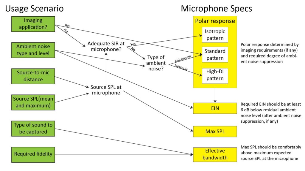
We’ll work backwards from each spec to see how they’re defined.

Maximum distortion-free SPL

This is the easiest spec to nail down; it’s determined by the maximum source SPL at the microphone diaphragm, which in turn is determined by the maximum source SPL at the source and the source-to-microphone distance.

A useful tool to help define the max SPL requirement is a plot of max SPL versus distance for various maximum source SPLs, as was previously presented in Figure 4 of this post.

Polar response

There are two application considerations that determine a microphone’s required polar response:

• Capturing multi-channel sound for an imaging format (such as stereo or Ambisonics) requires microphones with an anisotropic (directional) polar response, typically with a cardioid or figure-eight polar pattern.
• If the microphone isn’t going to be used to capture sound for an imaging format, then the required polar response is determined by the Signal-to-Interference Ratio (SIR) at the microphone.

The Signal-to-Interference Ratio (SIR)

The SIR is the ratio of the mean source SPL at the microphone to the ambient noise level. As shown in Figure 15, the concept is simple: we need a certain SIR_o at the microphone output for adequate sound quality, and if the SIR_i at the microphone input is too low, the microphone itself needs to suppress some of the ambient noise via its polar response:

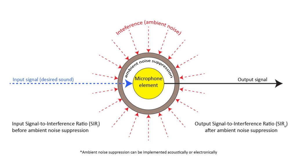
The required noise suppression is the difference between SIR_i and the required SIR_o.

The SIR at the microphone input

Assuming the variables are expressed in dB, the SIR_i at the microphone is the difference between the source SPL at the microphone (which, in turn, depends on the SPL at the source and the source-to-microphone distance) and the ambient noise SPL. The following figure plots curves of the source SPL at the microphone for typical sources, along with typical ambient noise levels:

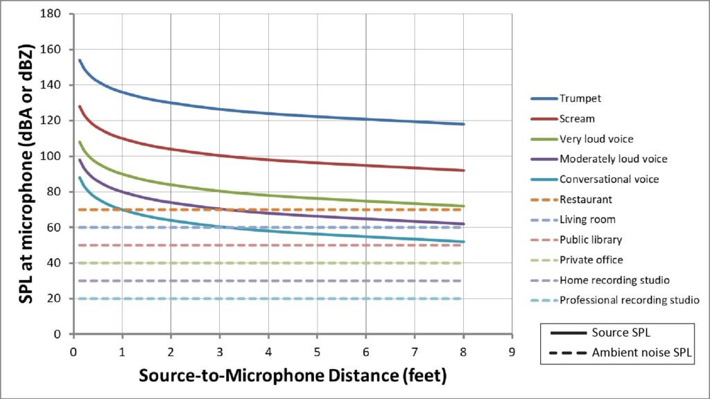
The SIR_i at the microphone is just the difference between the applicable solid (source) line and the applicable dotted (noise) line.

The required SIR at the microphone output

Obviously we want the SIR_o at the microphone output to be as high as possible, but how high is enough? That’s a subjective judgement and clearly depends on how the sound captured by the microphone is going to be used. I haven’t seen much discussion of this topic, but for what they’re worth, the SIR thresholds I myself use for various scenarios (based on my own experience and the limited info I’ve been able to find online) are summarized in the following table:

Minimum required SIR	Scenario
0 dB	Human voice barely/occasionally intelligible in some types of ambient noise. Potential threshold for being able to reliably recognize the presence of human voice in search-and-rescue scenarios (although unreliable recognition may be possible at SIRs as low as -6 dB)
8 dB	Assumed threshold of human voice intelligibility for surveillance applications (see long-range directional microphones)
12 dB	Wikipedia-cited threshold for 100 percent speech intelligibility [4]
20 dB	Minimum acceptable SIR for picking-up voice in conference room application (per Shure [5])
30 dB	Threshold for “good to excellent” speech intelligibility according to Shure [6]
40 dB	Threshold for high-quality pick-up of low-dynamic-range sound; minimum SIR benchmark for home recording studio
50 dB	Threshold for high-quality pick-up of high-dynamic-range sound; minimum SIR benchmark for professional recording studio

Required ambient noise rejection

As an example of the process used to determine the required ambient noise rejection, assume that we’re trying to capture moderately loud voice (80 dB SPL at a distance of 1 foot, per Figure 16) in a living room (with 60 dB SPL ambient noise, per Figure 16), and that we want “good to excellent” speech intelligibility (30 dB, per Table 6). The SIRi at the microphone input is 20 dB, but we need 30 dB…so the microphone must provide 10 dB of ambient noise rejection.

Required polar response versus required ambient noise rejection

Determining the required ambient noise suppression is straightforward, but translating it into a required microphone polar response can get complicated.

First let’s consider the two scenarios in which it’s not complicated: when the required suppression is no greater than 6 dB, and when the ambient noise is strongly anisotropic.

When 6 dB or less of ambient noise suppression is needed

From our discussion of polar patterns earlier in this post, we know that pressure-gradient (cardioid-family) microphones can provide a Directivity Index (DI) of up to 6 dB—and that the DI is doesn’t vary with frequency. So, if no ambient noise suppression is needed, we can just specify an isotropic response, and if up to 6 dB is needed, we can just specify a cardioid-family response, and be done with it.

When the ambient noise is anisotropic

When the ambient noise is coming mostly from one direction, then it’s not the DI that determines the achievable suppression; it’s the depth of the polar response’s null in the direction of the ambient noise.

Because of the nulls in their polar responses, cardioid microphones have a theoretically infinite ambient noise suppression at 180 degrees off-axis, while figure-eight (bidirectional) microphones have a theoretically infinite ambient noise suppression at 90 degrees off-axis. In practice, this is limited by the fact that some of the ambient noise gets reflected from nearby surfaces so that it’s not truly anisotropic (especially at low frequencies).

However, ambient noise is often anisotropic enough to get up to 20 dB of noise suppression with a cardioid or figure-eight pattern. Classic examples are suppressing crowd noises when recording live performances, avoiding feedback by suppressing the sound from speakers behind the microphone, and suppressing off-axis ambient noise while recording a one-on-one interview.

When more than 6 dB of suppression is needed and the noise is isotropic

This is where it gets complicated. When the noise is isotropic, it’s the Directivity Index (DI) that counts…and for practical microphone designs, DI’s of greater than 6 dB are always frequency-dependent.

To complicate things even further, ambient noise is also usually frequency-dependent and often heavily biased toward low frequencies.

The most conservative way to approach this from a specification standpoint is to require that the DI be equal to the required noise suppression at the lowest frequency of interest. However, such a requirement is usually impossible to meet with a practical microphone design. For example, let’s say that we need 10 dB of suppression, the lowest frequency of interest is 100 Hz, and we’re going to use the most directive type of microphone available for its size (a parabolic mic). A DI of 10 dB at 100 Hz would require a parabolic dish of over 10 feet in diameter, which certainly isn’t practical!

In addition to being impractical, such a conservative spec is overkill because because it’s based on the worst-case SIR over the microphone’s bandwidth, and therefore understates the overall SIR integrated over the entire bandwidth.

One practical way to get a more accurate estimate of the SIR for a microphone with a frequency-dependent DI is to:

• break-up the calculation into bandwidth chunks (I use octaves);
• calculate the SPL of the interference (as the product of the ambient noise SPL and DI) at each frequency;
• geometrically add the interference SPLs together to find the overall interference SPL over the bandwidth; and finally
• divide the signal SPL by the interference SPL to find the SIR.

This is a lot easier to do than it might seem, but is still beyond the scope of this discussion; I’m going to cover it in detail in an upcoming post. In the meantime, the main takeaway from this discussion is that suppressing isotropic ambient noise by much more than 6 dB isn’t easy and requires a specialized microphone.

Equivalent Input Noise (EIN)

In the preceding discussion on SIR, I intentionally omitted a variable for the sake of simplicity: it’s not just the interference (due to ambient noise) that competes with the desired signal; it’s also the EIN (self-noise) generated in the microphone. The preceding discussion assumes that the EIN is comfortably below the interference level so that it can be discounted in the SIR.

And, in fact, that’s how a microphone should be selected anyway: the EIN should be comfortably below the ambient noise level after any ambient noise suppression provided by the microphone. I strive for a margin of at least 6 dB between the residual ambient noise and the EIN, but I’ve come across recommendations as high as 10 to 15 dB (unfortunately I can’t recall the source of those recommendations).

Fortunately, it’s relatively easy to achieve this EIN criterion in almost any scenario, even with a DIY microphone.

Effective bandwidth

As previously discussed, a microphone’s required effective bandwidth depends on two factors:

• the range of frequencies in the sound to be captured, and
• the required fidelity of the output signal.

Ideally, the microphone’s effective bandwidth should span all of the frequencies in the sound to be captured, but a smaller bandwidth may be acceptable depending on the required fidelity, as previously shown in Table 5.

Final thoughts

Hopefully this discussion has given you a good understanding of the key microphone specs, how they affect overall performance, and how to choose them for a particular application.

Of course, if you expect to use the same microphone in many different typical usage scenarios, you might not want to optimize the specs for a given application. In that case, you’re going to want a high max SPL, a very low EIN, and a switchable polar pattern that offers a DI of up to 6 dB. You can build or buy such a general-purpose microphone, but understanding the importance of the specs is still important to build or buy the right one.

References

1. Brian C. J. Moore and Chin-Tuan Tan, “Perceived naturalness of spectrally distorted speech and music,” J. Acoust. Soc. Am. 114 (1), July 2003.  Available at https://www.academia.edu/6761417/Perceived_naturalness_of_spectrally_distorted_speech_and_music [accessed May 2022].
2. Gerald A. Studebaker, Chaslav A. Pavlovic, and Robert L. Sherbecoe, “A frequency-importance function for continuous discourse,”  J. Acoust. Soc. Am. 81 (4), April 1987. Available at https://www.researchgate.net/publication/19589656_A_frequency_importance_function_for_continuous_discourse [accessed May 2022].
3. Neville H. Fletcher, “A simple frequency-scaling rule for animal communication,” in J. Acoust. Soc. Am. 115 (5), Pt. 1, May 2004. Available at http://www.phys.unsw.edu.au/music/people/publications/Fletcher2004.pdf 2022].
4. Wikipedia contributors. “Intelligibility (communication).” Wikipedia, The Free Encyclopedia. Wikipedia, The Free Encyclopedia, 21 Feb. 2021. Web. 23 May. 2022.
5. Shure Corp., “Conference Room Acoustics and Signal-To-Noise Ratio,” https://service.shure.com/Service/s/article/conference-room-acoustics-and-signal-to-noise-ratio?language=en_US [accessed May 2022].
6. Shure Corp., “Predicting speech to background noise level at the microphone,” https://service.shure.com/s/article/predicting-speech-to-background-noise-level-at-the-microphone?language=en_US [accessed May 2022].