Predicting microphone performance—Part 2: using the SINR

In Part 1 of this post, I introduced the Signal-to-Interference-plus-Noise Ratio (SINR), explained why it’s the key microphone performance metric, and described how to calculate it. In this Part 2, I’ll discuss three ways of using the SINR for microphone performance prediction and present some SINR thresholds for various applications.

As I explained in Part 1 of this series, if we use a microphone properly (by ensuring that its maximum SPL isn’t exceeded and equalizing its output to provide the desired frequency response), then the only thing that will limit its performance is noise—both ambient noise (interference) and microphone self-noise. The SINR comprehends both types of noise, which is why it’s such a great performance metric.

However, there are two questions I didn’t address in Part 1:

• How much SINR is enough for typical microphone applications?
• The SINR can vary significantly with frequency over the bandwidth of interest. If it does, can a single SINR value still provide a useful measure of overall performance? Or, should we use multiple SINRs at various frequencies to gauge performance…and if so, how?

This post answers to both questions. By the way, I’ve never seen this topic addressed in this much detail anywhere else on the web.

Using a single SINR value to predict microphone performance

The simple way to quantify microphone performance is via just a single SINR value. We can obtain that value in one of three ways:

• We can evaluate the SINR over the whole bandwidth of interest (such as 20 Hz to 20 kHz for music, or perhaps 100 Hz to 8 kHz for voice). In fact, if you see a reference to an audio SINR (most often incorrectly labeled SNR, where the “N” includes not just microphone self-noise but also interference from ambient noise), it’s almost certainly referring to such a whole-bandwidth SINR.
• We can evaluate a frequency-specific SINR in a narrow sub-band centered at the frequency at which we expect the SINR to be the poorest over the bandwidth of interest.
• We can evaluate the SINR in a narrow sub-band centered at the frequency that we think has the greatest impact on the perceived quality of the captured sound.

All three approaches are compromises, but each can be useful in certain situations.

Using the SINR over the whole bandwidth of interest

The SINR isn’t used as a microphone performance metric as often as it should be, but when it is, it’s almost always the whole-bandwidth SINR, and it’s almost always based on SPLs that are A-weighted to account for the ear’s non-flat frequency response. Accordingly, most references to source and noise SPLs also cite whole-bandwidth values in dBA. For example, Wikipedia [1] provides the following examples of SPLs:

• “Normal conversation” at 1 meter: 40 – 60 dBA
• “Very calm room” (ambient noise): 20 – 30 dBA

These are whole-bandwidth values. If a studio microphone with an isotropic polar response and low self-noise (at least 6 dB or so less than the ambient noise) were used to pick up such a normal conversation in such a calm room, then the SINR at its output would be simply the source level minus the ambient noise level, or about 20 – 30 dB.

There are generally-accepted rules-of-thumb for the amount of whole-bandwidth SINR needed for various applications. Unfortunately, those rules-of-thumb aren’t (as far as I know) documented in any single place on the internet…until now, that is.

The following table—based on my own experience and scattered information I’ve been able to find online—lists some whole-bandwidth SINR rule-of-thumb for conventional studio microphones:

Minimum Bandwidth-integrated SINR at microphone output (based on A-weighted sound-pressure levels)	Subjective signal quality and potential applications
0 dB	Threshold for being able to detect the presence of voice or music, but insufficient to actually understand or recognize the sound
8 dB	Below-acceptable fidelity for quality-sensitive applications, but potentially suitable for surveillance applications where 100 percent speech intelligibility is not necessary (see long-range directional microphones)
12 dB	Poor fidelity, but still suitable for capturing intelligible voice when quality is not important. Wikipedia-cites 12 dB as the threshold for 100 percent speech intelligibility [2]
15 dB	Marginal fidelity: suitable for telecommunications applications. Note that Shure [3] cites 20 dB as the minimum acceptable SINR for picking-up voice in conference room applications
25 dB	Medium fidelity: suitable for business communications (such as videoconferencing, social media). Note that Shure [4] cites 30 dB as the threshold for “good to excellent” speech intelligibility
35 dB	High fidelity: suitable general-purpose professional applications (videography, podcasting, home recording studio)
45 dB	Maximum fidelity: suitable for the most demanding professional recording applications

However, an important caveat with the SINR benchmarks of Table 1 is that they’re valid only for microphones which:

• have a reasonably flat frequency response;
• have a reasonably flat directivity-versus-frequency characteristic; and
• are used in a typical indoor ambient-noise environment.

If a microphone application doesn’t meet these criteria, then the benchmarks of Table 1 don’t apply…and the whole-bandwidth SINR will give an inaccurate picture of the usefulness of the microphone’s output signal.

Unfortunately, many microphones for which performance prediction is especially important fall into this category. Notable examples include high-directivity microphones like shotgun or parabolic types. Because ambient noise usually decreases with frequency, all microphones usually have a SINR that increases with frequency, but that tendency is dramatically greater for such high-directivity microphones. Intuitively, it’s obvious that an extremely high SINR at, say 20 kHz wouldn’t make up for an unacceptably low SINR at, say, 2 kHz, so it’s evident that the whole-bandwidth SINR would overstate the performance of such a microphone.

Using the minimum SINR over the bandwidth of interest

An obvious way to avoid the performance overestimation that could occur with the whole-bandwidth SINR is to use the minimum SINR over the bandwidth of interest (which will almost always be the SINR at the lowest frequency over that bandwidth).

However, this is an ultra-conservative approach that will understate the actual signal quality too much to be useful for most applications, and I won’t discuss it further.

Using the SINR at the frequency of greatest importance

The concept of a “frequency of greatest importance” might seem to make little sense. After all, if we have a “bandwidth of interest”, shouldn’t all the frequencies in that bandwidth be equally important?

Not necessarily. Recall that we’re assuming that the microphone output will be equalized to yield the desired frequency response. So, all the signal frequencies we care about will be present in the microphone output in their proper proportions. The issue will be noise: the noise power won’t be flat with frequency, and it could too high at some frequencies for our application, which is the issue we’re trying to assess with our SINR prediction.

So, the “frequency of greatest importance” in this context refers to the frequency at which noise has the greatest impact on signal quality.

In fact, the concept of a “frequency of greatest importance” is actually pretty well-established for human voice: frequencies in the octave centered at ~2 kHz are known to contribute the most to vocal intelligibility, and noise in the same octave has a greater impact on perceived signal quality than noise at other frequencies.

Unfortunately, there is no such precedent for a “frequency of greatest importance” for music. However, studies involving voice suggest that much of the importance of frequencies around 2 kHz is due to the relatively high impact of noise at those frequencies, and it’s reasonable to assume that this would apply to music as well as voice. Therefore, it could be argued that the SINR in the octave centered at 2 kHz is a reasonable performance metric for both music and voice.

Thus, when the SINR is expected to vary a lot with frequency, the SINR in the 2 kHz octave is probably a better measure of microphone performance for both voice and music than the SINR over the whole voice or music bandwidth. Since the A-weighted SPL at 2 kHz is only 1.2 dB greater than the unweighted value, it makes little difference if the 2 kHz SINR is based on A-weighted variables (in dBA) or unweighted variables (in dBZ).

Unfortunately, as far as I know, there have been no studies to determine how high such a “2 kHz SINR” needs to be for various applications.

Also, while 2 kHz (or some nearby frequency) might be the most important frequency, it’s obviously not the only important frequency. If a signal has a very low SINR at other frequencies, then a metric based on just the most important frequency will still overestimate the overall signal quality.

Using multiple SINR values to predict microphone performance

The obvious solution to the limitations of a performance metric based on a SINR value is one based on SINRs at multiple frequencies.

But how do we combine multiple SINRs into a single metric, and how do we quantify the relationship between that metric and microphone signal quality? Fortunately, an existing sound-quality metric used by audiologists—known as the Articulation Index (AI)—points the way.

There’s a lot of information online on the AI (see for example [5]), so I’m not going to describe it in much detail; rather, I’ll just give a brief overview and then focus on how the AI can be adapted for predicting a microphone’s voice pick-up range.

A brief introduction to the Articulation Index (AI)

The AI was originally developed at Bell Telephone Laboratories in the late 1940s for telecommunications engineering applications, but was soon adopted by audiologists to help quantify the impact of hearing loss (and is still being used today for that purpose).

The AI is based on the ear’s SNR, not a microphone SINR

Before we get into the AI, we need to understand the difference between three commonly-cited ratios of signal to noise:

• There is the microphone SINR we’ve been discussing, in which the “noise” term includes both acoustic interference and microphone self-noise. So, the noise term represents the net effective noise (the noise “floor”) that competes with the signal.
• There is the SNR as used in microphone specifications, in which the noise term includes only the microphone self-noise. Also, unlike the SINR, the signal term in this SNR is always a fixed reference signal of 94 dBA (see my post on the 4 key microphone specifications for more info on this flavor of SNR).
• And finally, the AI as used conventionally is based on a different SNR, in which the noise term includes both ambient noise (acoustic interference) and the ear’s self-noise. So, as with the SINR, the noise term of this SNR represents the net effective noise that competes with the “signal” at the output of the ear.

Thus the SNR as used in the AI, and the SINR we’ve been discussing, are effectively equivalent for our purposes because they both describe the margin between a desired signal level and a competing noise floor. The only difference is that the SINR applies to microphones (hence the inclusion of microphone self-noise), whereas the AI’s SNR applies to the ear (hence the inclusion of the ear’s self-noise instead of microphone self-noise).

The AI is effectively a weighted sum of SNRs

The AI is based on the idea that the contribution of each frequency to overall speech intelligibility can be estimated as a linear function of the ear’s output SNR (in dB) at that frequency, multiplied by the relative importance of that frequency. The AI is thus a weighted sum across multiple frequency sub-bands:

• AI = Σ(I_iA_i), where:
  • Σ is a summation over a number of frequency sub-bands that span the vocal bandwidth and i represents the band index. Historically, the number of sub-bands has ranged from 4 to 21, but today 16 one-third-octave sub-bands are typically used, spanning a bandwidth of 200 Hz to 6.3 kHz.
  • I_i is the weighting value for sub-band i based on a frequency importance function. The weights are such that their sum over all the sub-bands equals 1.0. Note that these weights take into account the ear’s non-flat frequency response.
  • A_i is an audibility factor, ranging from 0.0 to 1.0, that determines how much of the SNR at sub-band i actually contributes to the overall AI. The audibility factor is determined by a linear audibility function of the SNR in dB, such that an SNR of 0 dB results in an A_I of 0.0, and an SNR of 30 dB results in an A_I of 1.0. Because the frequency importance function accounts for the ear’s non-flat frequency response, the SNR is calculated using unweighted sound pressure variables.

Thus, the overall AI also ranges from 0.0 to 1.0. This AI value is correlated with speech intelligibility, but doesn’t directly represent an intelligibility percentage. An actual intelligibility percentage is important in audiology because it expresses hearing loss in terms a patient can understand. So, the AI value is typically converted into an intelligibility percentage by means of an intelligibility transfer function.

There is a key difference between this AI approach and the whole-bandwidth SINR approach (described previously in connection with Table 1) that’s worth emphasizing:

• In the AI approach, the contribution of each sub-band’s SINR to the overall metric is determined by just the frequency-importance and audibility functions, and does not depend on the absolute width (in Hz) of each sub-band.
• In contrast, in the whole-bandwidth SINR, the SINR at lower octaves contributes much less to the overall SINR than the SINR at higher octaves. That’s because the lower octaves are much narrower (in Hz) than the higher octaves, and signal power is proportional to bandwidth.

As a result, the AI metric can be more sensitive to SINR deficits at lower frequencies (depending on the frequency importance function) than the whole-bandwidth SINR, which makes it a better indicator of actual signal quality.

The next paragraphs describe key aspects of the AI in more detail.

The frequency-importance function

The frequency-importance function reflects the relative importance of the SNR in each sub-band.

Many frequency importance functions have been developed for conventional AI applications. Such a function is obtained by measuring the ability of test subjects to correctly understand frequency-filtered syllables, words, and sentences. Two such functions are shown in the figure below:

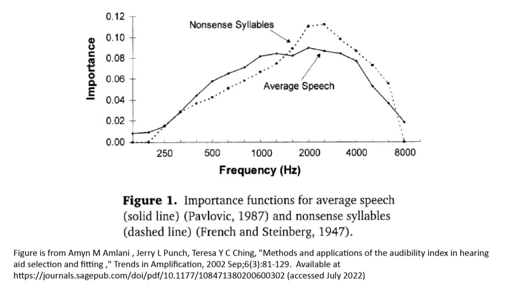
When looking at these curves, recall that the ordinate represents the weight (or relative importance) of the SNR at the frequency indicated by the abscissa, and that the weights of all of the center frequencies (sub-bands) must sum to 1.0. These particular importance functions are based on eighteen sub-bands, which is why the ordinate values are so small.

The curves of Figure 1 show why 2 kHz can be taken as “the most important frequency” for voice intelligibility, and that frequencies around 2 kHz are especially important when recognizing nonsense syllables versus average speech. The reason for the differences in the shapes of the curves is that average speech provides contextual cues that increase the intelligibility of each word, while nonsense syllables do not—and those contextual cues apparently reduce the relative importance of the SNR at frequencies near 2 kHz.

You might be surprised that the curves of Figure 1 ascribe so little importance to frequencies below 500 Hz and above 4 kHz. Indeed, as I discuss in the bandwidth section of my post on the four key microphone specifications, frequencies as low as 60 Hz and as high as 17 kHz contribute significantly to the perceived naturalness of voice and music. The discrepancy is due to the fact that importance functions like those shown in Figure 1 are aimed at obtaining an estimate of voice intelligibility, not naturalness or fidelity.

The audibility function

The audibility function determines how much of the SNR in a given sub-band actually contributes to the AI. In conventional AI metrics, the audibility function is based on two assumptions:

• A given sub-band won’t contribute at all to speech intelligibility (in other words, A_i will be 0.0) when the speech SPL is at or below the hearing threshold at that frequency. The hearing threshold is effectively the ear’s self-noise, analogous to a microphone’s Effective Input Noise (EIN).
• A given sub-band will make its maximum contribution to speech intelligibility (in other words, A_i will be 1.0) when the speech SPL at that frequency is 30 dB greater than the hearing threshold at that frequency.

So, the conventional audibility function is a linear mapping between an SNR range of 0-30 dB and an audibility range of 0.0-1.0, as shown in the following figure:

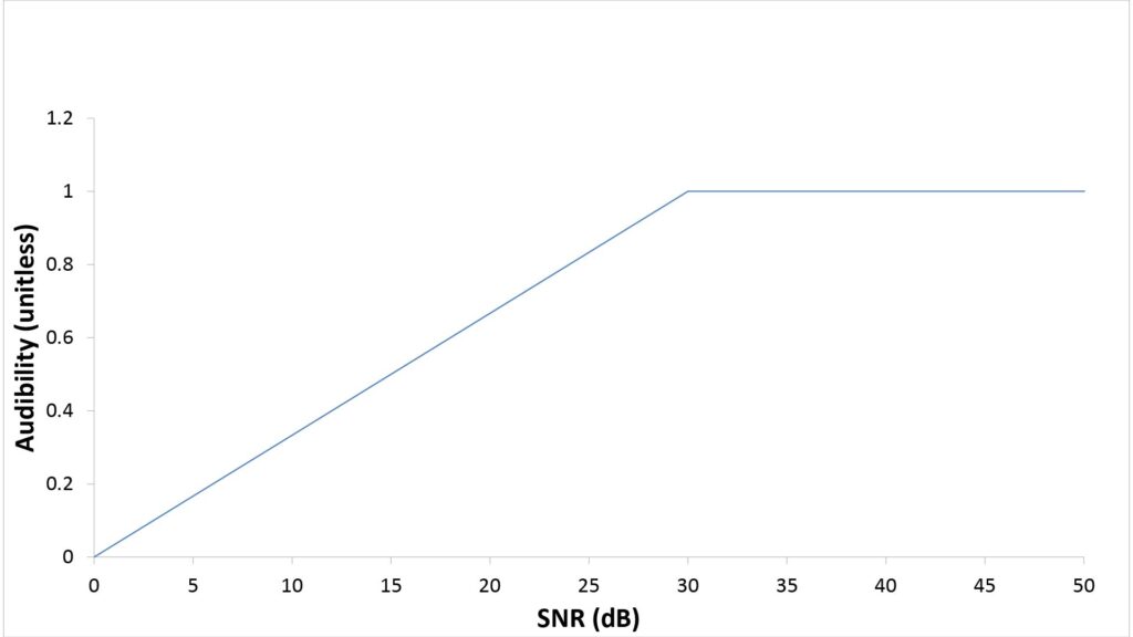
The fact that a conventional audibility function doesn’t address SNRs below 0 dB makes sense because sounds at or below the ear’s hearing threshold are (by definition) inaudible. And the fact that no benefit is ascribed to SNRs above 30 dB also makes sense, because there is no such thing as speech that is more than 100 percent intelligible.

The Intelligibility transfer function

In conventional AI metrics, an AI of 100 percent corresponds to 100 percent voice intelligibility, while an AI of 0 percent corresponds to 0 percent voice intelligibility. However, there isn’t a one-to-one correspondence between AI and intelligibility for intermediate values of AI. Instead, an intelligibility transfer function is necessary to convert the AI value to an actual intelligibility percentage.

Googling “speech intelligibility transfer function” or “articulation index transfer function” will yield several examples of such functions if you’re interested. The following figure, from Amlani at al [5], shows several intelligibility transfer functions:

Note that the shape of the function depends on the type of speech in question:

• For types of speech that provide contextual cues (such as complete sentences), an AI of 50 percent can still yield an intelligibility exceeding 80 percent. In fact, for this type of speech, the AI has to fall below about 20 percent before the intelligibility drops below 50 percent.
• The intelligibility is obviously lower for a given AI if the speech doesn’t provide contextual cues (as is the case with random words or nonsense syllables). However, intelligibility still typically exceeds 50 percent when the AI is 50 percent.

Obviously, the estimated intelligibility percentage is very useful for counseling individuals with hearing loss, but isn’t always necessary in the context of a general-purpose microphone performance metric. More on that later.

Adapting the AI for use as a microphone performance metric

The conventional AI as described above could be used almost as-is as a microphone performance metric for applications which stress speech intelligibility (such as surveillance or telecommunications). However, there are modifications which can make it easier to use for intelligibility-intensive applications and extend its applicability to fidelity-sensitive applications.

Using full-octave rather than third-octave sub-bands

The third-octave bands used in the conventional AI are overkill for microphone performance prediction; the metric is a lot easier to use (with very little loss in accuracy) with fewer and wider bands. Specifically, I use full-octave sub-bands which provide sufficient granularity for microphone performance characterization and make the calculations a lot easier.

Extending the metric for fidelity-intensive applications

The conventional AI has three obvious limitations when fidelity—and not just intelligibility—is the driving requirement:

• A given sub-band’s contribution to intelligibility isn’t necessarily the same as its contribution to fidelity. For example, low and high frequencies that aren’t important for speech intelligibility still have a significant effect on the perceived naturalness of both speech and music.
• The conventional AI is intended to “max out” at 100 percent speech intelligibility, whereas some noise can still be audible with 100 percent intelligibility. So, we would expect the perceived quality of speech (as well as music) to keep increasing with SINR beyond the 30 dB required for 100 percent speech intelligibility.
• There isn’t a generally-accepted “fidelity transfer function”, analogous to the intelligibility transfer function, that can convert a weighted sum of sub-band SINRs into a useful measure of fidelity.

So, three modifications are needed to extend the AI approach for fidelity-intensive applications:

• The importance function (previously shown in Figure 1) must be changed to reflect the relative importance of each sub-band to fidelity rather than to intelligibility.
• The audibility function (previously shown in Figure 2) must be extended so that it assigns credit for SINRs greater than 30 dB.
• Some kind of “fidelity transfer function” is needed.

Ideally, such modifications would be based on an extensive test program involving a large number of people. Lacking the resources for such a test program, I’ve used a heuristic approach to develop a modified AI-style metric that seems to work pretty well for both intelligibility-sensitive and fidelity-sensitve applications…and that’s the subject of the next section.

Using a weighted-SINR quality metric optimized for microphone performance prediction

So far, this post has explained the limitations of a single SINR value in characterizing microphone performance and has discussed how a metric using multiple SINRs, based on the Articulation Index (AI), can be leveraged to overcome those limitations. In this section I’ll describe two such metrics that I use for my microphone analyses.

The two metrics, which I call the Fidelity Index (FI) and the Intelligibility Index (II), are essentially the same as the Articulation Index except for a few minor differences. They’re calculated as follows:

• FI or II = Σ(I_iA_i), where:
  • Σ is a summation over eleven octave-wide sub-bands, with center frequencies ranging from 16 Hz to 16 kHz.
  • I_i is the weighting value for sub-band i based on one of two frequency-importance functions; one importance function is used for the II and the other for the FI.
  • A_i is one of two audibility functions of the SINR in dB for sub-band i; one audibility function is used for the II and other for the FI. The SINR is calculated as described in Part 1 of this series, except that it requires that the sound-pressure values be unweighted rather than A-weighted.

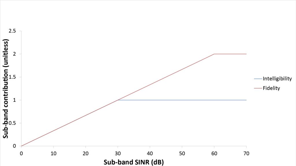
Figures 4 and 5 show the two frequency-importance and audibility functions:

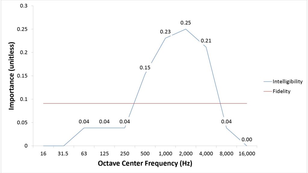
A few aspects of these functions merit a bit more explanation:

• The importance function used for the Intelligibility Index (II) is the same as that used in the conventional AI (except that the weights have been adjusted to reflect the smaller number of sub-bands): it weights each sub-band according to its importance for speech intelligibility.
• In contrast, the importance function used for the Fidelity Index (FI) weights each sub-band equally. This is based on nothing more than intuition (a flat weighting “seems right” for a fidelity-oriented metric), but it works well in practice.
• The audibility function used for the II is the same as that used in the conventional AI; it assigns credit for only up to 30 dB of sub-band SINR.
• On the other hand, the audibility function used for the FI assigns credit for up to 60 dB of sub-band SINR. I developed this using a mixture of heuristics and testing; I can’t guarantee that it’s optimum, but it too seems to work pretty well in practice.

How the metric relates to speech intelligibility

After the value of the Intelligibility Index (II) is obtained using the corresponding audibility and importance functions shown in Figures 4 and 5, it can be used in either of two ways.

First, it can be converted into an intelligibility percentage using the intelligibility transfer function shown in Figure 6:

This function is essentially identical to one commonly used in audiology applications for “whole sentence” intelligibility. Note that the intelligibility percentage becomes insensitive to II when II is above 0.4 or so, whereas we would expect the perceived quality (although not the intelligibility) of speech to increase up to a II of 1.0. Therefore, the transfer function of Figure 6 is most useful when we’re interested in applications in which marginal intelligibility is acceptable, such as long-distance surveillance.

On the other hand, if we’re interested in high-quality voice pickup, then we can either use the Fidelity Index (FI) described in the next paragraph instead of II or we can use the following table instead of the transfer function of Figure 6:

Minimum value of Intelligibility Index	Quality of speech-oriented output signal
0.1	Extremely poor; intelligibility of ~20%, but suitable for detecting the presence of speech in noise (such as for detecting shouts from lost parties in search-and-rescue applications)
0.25	Poor: intelligibility of ~80% for complete sentences (but only ~25% for nonsense syllables) with heavy audible noise.
0.5	Modest: intelligibility of ~90% but with significant audible noise; suitable for general-purpose speech-capture applications
0.75	High: intelligibility of ~100% for complete sentences and 90% for nonsense syllables; suitable for all but the most demanding speech-capture applications
1.0	High: intelligibility of 100% for both speech and nonsense syllables; suitable for the most demanding speech-capture applications

How the metric relates to sound fidelity

If we’re interested in a fidelity-sensitive application, when we would use the corresponding audibility and importance functions shown in Figures 4 and 5 to obtain the Fidelity Index (FI)

Unfortunately, there is no recognized “fidelity transfer function” to translate FI into a quantitative fidelity metric. Instead, we can use the following table to translate the value into qualitative fidelity thresholds:

Minimum value of the Fidelity Index	Fidelity of output signal
0.5	Poor fidelity but potentially useful in capturing speech for undemanding communications or social media applications (in which case qI may be a more appropriate metric)
0.8	Medium fidelity; suitable for general-purpose communications and social-media applications
1.2	High fidelity; suitable for all but the most demanding applications, including podcasting and videography
1.5	Maximum fidelity; suitable for professional recording applications

How accurate is such a quality metric?

There are two short answers to this question:

• it’s accurate enough to be useful; and
• it’s more accurate than any other simple method I’m aware of to quantify the quality of a microphone’s output signal.

Of course, there are also longer answers.

Relative accuracy

One of the most useful applications for a metric like this is to gauge the quality of the signal produced by a particular microphone relative to that of a known microphone.

For example, suppose that we know, from experience, the quality of the signal produced by a lavalier microphone that’s 12 inches from a speaker’s mouth in a home recording studio. Suppose also that we’re considering buying a particular shotgun microphone to replace the lavalier, but need to know if the shotgun’s increased range would justify its cost.

We can answer this question by first determining the signal quality for the lavalier, and then solving for the range at which the shotgun provides the same signal quality. In this case, we don’t need an accurate estimate of the absolute quality of the microphones’ output signals (in other words, we don’t need an accurate estimate of speech intelligibility or sound fidelity). In this case, then, the accuracy of the intelligibility function of Figure 6, or the quality thresholds of Tables 2 or 3, aren’t important.

What is important, however, is that our quality metric produce roughly the same value for both the lavalier and shotgun outputs when they have the same subjective signal quality.

My experience has been that the quality metric described above has more than enough relative accuracy to answer questions like this.

Absolute accuracy

On the other hand, suppose that we don’t have any experience with the sound quality of an actual microphone in a given location, but still want to know how well a particular microphone will work in that location.

In this case, the absolute accuracy of the intelligibility or fidelity prediction of our metric is important, and so therefore are the accuracies of the intelligibility function of Figure 6 and quality thresholds of Tables 2 and 3.

However, even in this case I think the model is more than accurate enough to be useful, particularly for intelligibility-sensitive applications involving speech. That’s because the Intelligibility Index and intelligibility transfer function described above are virtually identical to those proven over decades of use in audiology applications.

In any case, the metric is still certainly more accurate than the conventional way of using the whole-bandwidth SINR to predict microphone performance.

Potential applications of a SINR-based microphone performance metric

Once we have a SINR-based performance metric, how can we use it? Here are just a few:

• Predicting the pick-up range of long-distance microphones like parabolic and shotgun types.
• Determining the required maximum SPL-handling capability of a studio microphone. We can do this by first determining the maximum allowable distance between the microphone and the source for the desired SINR-based signal quality, and then predicting the maximum SPL at that distance.
• Determining the maximum allowable microphone self-noise for a given usage scenario.
• Determining the maximum allowable ambient noise level for a given usage scenario.

References

1. Wikipedia contributors. “Sound pressure.” Wikipedia, The Free Encyclopedia. Wikipedia, The Free Encyclopedia, 13 Jul. 2022. Web. 15 Aug. 2022.
2. Wikipedia contributors. “Intelligibility (communication).” Wikipedia, The Free Encyclopedia. Wikipedia, The Free Encyclopedia, 8 Jul. 2022. Web. 15 Aug. 2022.
3. Shure Corp., “Conference Room Acoustics and Signal-To-Noise Ratio,” https://service.shure.com/Service/s/article/conference-room-acoustics-and-signal-to-noise-ratio?language=en_US (accessed May 2022).
4. Shure Corp., “Predicting speech to background noise level at the microphone,” https://service.shure.com/s/article/predicting-speech-to-background-noise-level-at-the-microphone?language=en_US (accessed May 2022).
5. Amyn M Amlani , Jerry L Punch, Teresa Y C Ching, “Methods and applications of the audibility index in hearing aid selection and fitting ,” Trends in Amplification, 2002 Sep;6(3):81-129. Available at https://journals.sagepub.com/doi/pdf/10.1177/108471380200600302 (accessed July 2022).