How horn microphones work

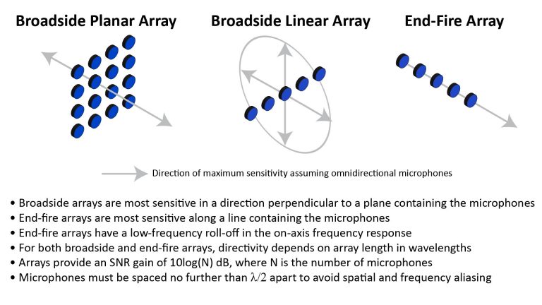
Not many people have ever heard of horn microphones (much less know how horn microphones work), but they’re potentially great alternatives to parabolic and shotgun microphones. They offer some unique performance advantages (but also have some unique limitations), while also being easier and cheaper to fabricate.

A horn microphone works like a cheerleader’s megaphone, but in reverse: sound arriving at the mouth of a horn is concentrated at its throat, where the concentrated sound is sensed by a microphone element. This concentration effect provides acoustic gain, while the large mouth area and flaring sidewalls provide wavelength-dependent directivity.

While the operation of a horn megaphone or microphone is intuitively simple, the underlying theory can get quite complex. Fortunately, a complete understanding of the theory isn’t necessary in order to understand or even build an effective horn microphone, as long as you have a grasp of the basic principles and are aware of a few important design considerations. That’s what I’m going cover in this post.

Introduction to horn microphones

The horn microphone is a deceptively simple device: it consists of a conventional microphone element mounted at the throat of a horn, which is just a flared tube whose cross-sectional area increases with distance from a narrow throat to a wider mouth.

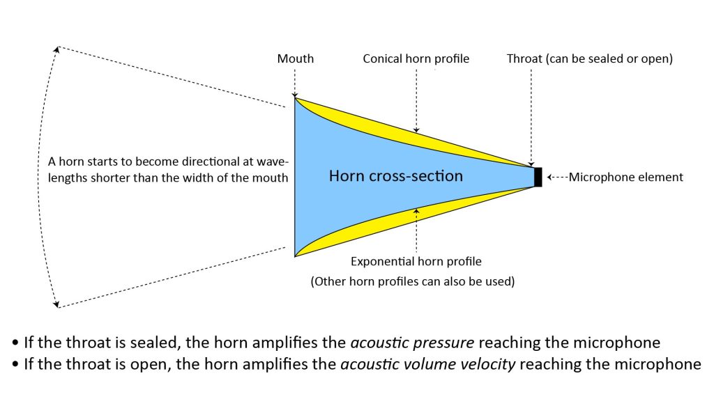
The mathematical function that expresses how the cross-sectional area increases with distance from the throat is referred to as the horn profile. The figure shows just two profiles (conical and exponential), but many other profiles can be used, each with their own trade-offs.

The horn microphone does what you’d expect it to do: it amplifies the sound that reaches the microphone element, and it makes the microphone element more directional. If the throat of the horn is sealed, the horn amplifies the acoustic pressure reaching the microphone; if the throat is open, the horn amplifies the acoustic volume velocity reaching the microphone.

But how a horn microphone does these things, and how well it does them, is not quite so simple. We’ll get into that later.

The earliest useful microphones were horn microphones

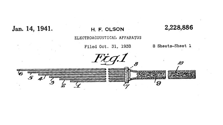
The first microphones capable of converting sound into a useful electrical signal were, in fact, horn microphones. For example, the first true microphone was arguably the device disclosed by Alexander Graham Bell in his seminal U.S. patent 174,465 of March 7, 1876 for “Improvement in Telegraphy” (which actually described an early version of his telephone)…and this was clearly a horn microphone:

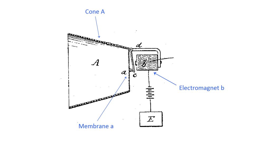
Bell’s microphone might have used a horn because his microphone element (an early form of dynamic microphone) wasn’t sensitive enough to produce a useful signal; Bell’s solution was to use a cone (which is a type of horn) to amplify the sound reaching the diaphragm (or “membrane” in Bell’s parlance).

Why horn microphones aren’t as common as horn speakers

You’re probably already familiar with horn speakers and know that they’re pretty widely used today. But you might have never heard of horn microphones before reading this post…and if you have, it was probably just in a historical context.

So, since horn microphones work in exactly the same way as horn speakers (except in reverse), why aren’t they as common as horn speakers?

There are two reasons.

First, the ability of a horn microphone to amplify sound is much less relevant today than in Alexander Graham Bell’s time, because modern microphone elements already offer more than enough sensitivity and a low-enough self-noise for most applications. Conversely, the sound amplification function of a horn will always be relevant for certain speaker applications, because it can dramatically increase speaker efficiency (in terms of the sound volume produced per watt of amplifier power).

Second, the value of the horn’s ability to make a microphone element more directional is tempered by the availability of other types of directional microphone…specifically the shotgun and parabolic types.

But does that mean that horn microphones are no longer relevant? Not at all!

Why horn microphones are still relevant

While horn microphones are no longer relevant for general use, they offer some unique advantages (but also some unique disadvantages) in long-range applications. In fact, depending on the specifics of the application, a horn microphone can be a better choice than either a shotgun or parabolic microphone.

I have a detailed comparison of various types of long-range microphones at How long-range microphones work, so here I’ll just mention what is probably the biggest advantage of horn microphones: they’re easier and less expensive to build than other types of highly directional microphone. A horn mic won’t provide the same reach as a comparably-sized parabolic mic and will be harder to handle than a shotgun mic, but for some applications it might be just right.

In fact, my research has convinced me that horn microphones are greatly underappreciated, especially in the DIY community.

BTW, check out these other posts for information on alternatives to horn microphones:

• A deep look at how shotgun microphones REALLY work
• How array microphones work
• The complete guide to parabolic microphones

The two fundamental types of horn microphone

As alluded to in the introduction, there are two fundamental types of horn microphone:

• An Acoustic Pressure Horn (APH) microphone amplifies the acoustic pressure at the microphone element.
• Conversely, an Acoustic Velocity Horn (AVH) amplifies the acoustic volume velocity at the microphone element.

The APH has been studied extensively (mainly for speaker applications) for almost a century, while the AVH is relatively new on the public scene (first appearing in the technical literature in 2011). For this and other reasons, virtually all horn microphones—and literally all horn speakers—have used the APH configuration. However, the AVH is an interesting and seemingly useful device for certain microphone applications.

From a physical standpoint, the distinctions between an APH and an AVH are straightforward: an APH has a sealed throat and uses a pressure microphone element, while an AVH has an open throat and uses a pressure-gradient microphone element.

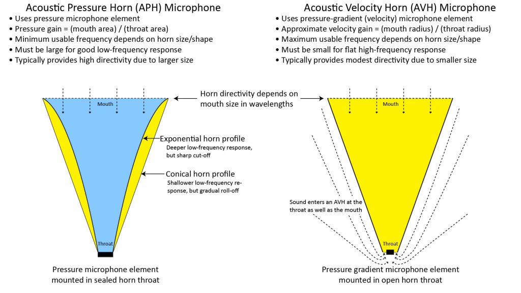
However, from an analytical standpoint, the APH and AVH are radically different devices. The fact that sound can enter an AVH from both the mouth and the throat means that the physics inside the horn are completely different, and that the century’s worth of accumulated understanding of the APH isn’t applicable to the AVH.

I’ll describe APH and AVH microphones in more detail later, but the accompanying table lists some highlights.

Acoustic Pressure Horn (APH) Microphone	Acoustic Velocity Horn (AVH) Microphone
Uses pressure microphone	Uses pressure-gradient microphone
Amplifies acoustic pressure at the throat	Amplifies acoustic volume velocity at the throat
Pressure gain is equal to ratio of mouth area to throat area	Velocity gain is approximately equal to ratio of mouth radius to throat radius
Provides unidirectional directivity	Provides bidirectional (dipole) directivity
Works well at higher frequencies: minimum usable frequency is limited by horn reactance; no practical upper-frequency limit in most applications	Works well at lower frequencies: maximum usable frequency is potentially limited by fundamental horn resonance; no practical lower-frequency limit in most applications.
Horn must be large to work well at bass frequencies	Horn must be small if it is desired to keep fundamental resonant frequency above voice spectrum
Provides extremely high gain and high directivity when sized to work well at voice frequencies	Provides modest gain and only dipole directivity when sized to keep fundamental resonance above voice frequencies; can provide significant gain and a sharp bidirectional polar pattern if operated above fundamental resonant frequency
Best for: picking-up voice and wildlife sounds at long range (offers longer range than shotgun mics while being easier to build than parabolic mics)	Best for: specialized studio microphones, specialized low-frequency applications (low-frequency direction-finding, infrasonic sensing)

As you can see from the table, APH and AVH microphones are very different devices, but both are potentially very useful.

A closer look at Acoustic Pressure Horn (APH) microphones

As mentioned in the introduction, virtually all horn microphones and literally all horn speakers use an Acoustic Pressure Horn (APH). So, if the type of horn (APH versus AVH) isn’t specified—and it rarely is—you can safely assume that a horn microphone or a horn speaker is using an APH.

Because APH speakers were originally the only type of practical speaker available and are still widely used today, there is plenty of information online about how they work and how to design them. Fortunately, much of that information is directly applicable to horn microphones.

The classical and modern frameworks for understanding the APH

In the introduction, I mentioned that the horn in a horn microphone or speaker performs two functions: it increases the directivity of the transducer, and it amplifies the sound received or emitted by the horn.

Until the turn of the century (the 21st Century, that is), these two functions of an APH were generally understood and analyzed separately, using two theoretical frameworks: one which deals with what happens inside the horn (which addresses the horn’s ability to amplify sound), and one which deals with what happens outside the horn (which addresses directivity). This approach enables prediction of approximate APH behavior using relatively simple equations, which was crucial in the days before computers.

However, the preferred approach since the early 2,000’s has been to use numerical techniques such as Finite-Element Analysis (FEA) and the Boundary Element Method (BEM) to analyze the interior and exterior behavior of horns holistically. These techniques can predict horn performance (especially far-field directivity) more accurately than the classical approach.

However, there’s a pretty steep learning curve in applying such numerical techniques, and they don’t provide as much insight into horn operation as the classical approach. So, while I’ll link to some references that address numerical techniques, the rest of this post is going to focus on the classical approach to understanding APH operation.

The classical approach to analyzing what happens inside an APH

The classical approach to analyzing the APH was developed at a time when amplifier power was very expensive, so maximizing speaker efficiency was crucial.

Accordingly, the main function of the horn in early horn speakers was to match the relatively high acoustic impedance of a speaker driver with the relatively low acoustic impedance of free-space, greatly increasing the SPL produced per watt of amplifier power. Dinsdale [1] also cites the reduced driver excursion per unit SPL (which reduces distortion due to nonlinearities) as another key benefit of the high efficiency of horn speakers.

Thus, the classical approach was centered on this ability of a horn to serve as an acoustic impedance transformer.

The APH as an acoustic impedance transformer

Acoustic impedance is analogous to electrical impedance: it represents the opposition of a device or medium to acoustic volume velocity (analogous to electrical current) caused by acoustic pressure (analogous to voltage). In other words, acoustic impedance is equal to pressure divided by volume velocity.

Free space (air) is considered to have a low acoustic impedance because it provides little opposition to acoustic pressure: when a speaker tries to apply pressure to air, that pressure is instantly translated into volume velocity. Conversely, a speaker has a high acoustic impedance because it can only produce acoustic power to the extent that it can “push” against something. A pressure microphone also has high acoustic impedance because it responds to pressure rather than volume velocity.

So, the APH in a horn speaker functions as a step-down acoustic impedance transformer, transforming a high impedance at the throat (high ratio of pressure to volume velocity) to a lower acoustic impedance at the mouth (lower ratio of pressure to volume velocity. Conversely, the APH in a horn microphone can be viewed as a step-up acoustic impedance transformer, transforming a low impedance at the mouth to a high impedance at the throat.

Just as with electrical power, transfer of acoustic power across an interface is maximized when each side of the interface has the same impedance. That’s why an APH can significantly increase the efficiency of an acoustic transducer, such as a compression driver or pressure microphone, whose acoustic impedance is significantly greater than that of free space (air).

However, a horn has its own impedance, and if the horn itself introduces an impedance mismatch, then some of the power arriving at the mouth won’t reach the throat. In fact, under certain conditions a horn can, in theory, completely block the transfer of power between the mouth and throat.

Acoustic impedance is a complex quantity

Like electrical impedance, acoustic impedance is a complex quantity that can include both a real component (acoustic resistance) and an imaginary component (acoustic reactance). If the acoustic pressure and volume velocity are in phase, then there is no reactance and the acoustic impedance is just the ratio of the volume velocity to the acoustic pressure. This is the case with free space. However, if the volume velocity and pressure are not perfectly in phase, there is a reactive component and the magnitude of the resistive component is reduced.

Only the resistive component of a device’s or medium’s impedance can supply or dissipate power. Acoustic reactance temporarily stores, but then later returns, power over the period of the time-varying pressure and velocity waveforms.

Therefore, efficient transfer of acoustic power across an interface requires that the impedance on both sides of the interface are purely resistive and of the same magnitude. Otherwise, some of the power will be reflected back to the source.

A horn’s mouth and throat become reactive at lower frequencies

A horn’s mouth and throat each have their own acoustic impedance. So, there are actually two impedance interfaces in a horn used with an acoustic transducer: the free-space-to-mouth interface, and the transducer-to-throat interface.

A major issue with horn operation is that, as the frequency drops below values that depend on the horn design, either or both the mouth and throat impedance can become reactive instead of resistive. When that happens, some of the sound power arriving at the mouth or throat, respectively, will be reflected back to the source.

Reactance at either the mouth or throat is bad not only because it reduces the power transfer efficiency, but also because the resulting power reflection causes standing waves within the horn, which in turn induce ripples in the frequency response.

The frequency at which the mouth resistance drops and its reactance rises is called the mouth cutoff frequency, while the frequency at which the throat resistance drops and its reactance rises is called the throat cutoff frequency.

Although these are referred to as “cutoff” frequencies, neither the horn nor mouth of an APH abruptly stops transferring power below the corresponding cutoff. As we’ll see later, the throat cutoff can be either quite sharp or gradual, depending on the horn design.

Determining APH throat impedance versus frequency

For the reasons outlined above, an APH’s throat-resistance-versus-frequency curve is traditionally considered to be a proxy for its frequency response. So a key objective in classical APH analysis is to predict the throat impedance, and especially its resistive component, as a function of frequency. This is done by solving Webster’s Horn Equation.

Webster’s Horn Equation

In the days before computers, the only way to solve complex problems was via purely analytic techniques; modern numerical techniques simply weren’t an option.

However, modeling the pressure and velocity fields inside a horn of arbitrary shape is a three-dimensional problem, which makes a purely analytical solution prohibitively complex. So the early developers of horn theory had to resort to making some simplifying assumptions (along with a lot of creativity) in an effort to analyze horn behavior. Webster’s Horn Equation (which I’ll abbreviate as the WHE) was the result.

While the WHE is attributed to Arthur Gordon Webster for his 1919 paper [2] on phonograph horns, the WHE wasn’t actually originated by Webster. However, he was arguably the first to apply it to the problem of analyzing the acoustic impedance of practical horns. See Eisener [3] and Section 2.2 of Morgans [4] for a discussion of the history of horn theory, Webster’s place in it, and other major contributors to the field.

The WHE is based on the simplifying assumption that sound propagates inside a horn as a plane wave with uniform pressure across the horn’s cross-section. This turns the problem of finding the horn’s throat impedance into a one-dimensional differential equation that has an exact solution for many types of horn.

Applying Webster’s Horn Equation: infinite versus finite horns

While solving the WHE can yield an exact expression for the throat impedance for many types of horn, that expression isn’t necessarily simple. One reason is that is that, in all real horns, the throat impedance depends on the mouth impedance, making the solution a bit cumbersome.

The solution can be simplified by assuming that the subject horn is infinitely long. This infinite horn assumption doesn’t necessarily mean that the actual length of the horn isn’t considered in the solution for the throat impedance, but it does mean that interactions between the horn’s mouth and throat are ignored.

The finite-horn and infinite-horn approaches to using the WBE to model throat impedance are illustrated in Figure 4:

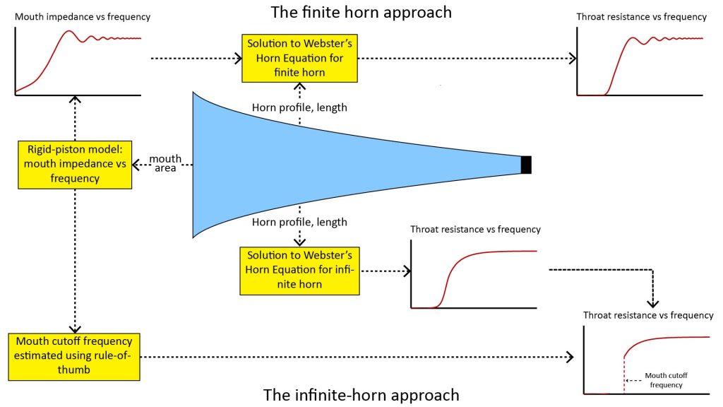
The classical finite horn approach

As shown at the top of Figure 4, the finite horn approach obtains the throat impedance versus frequency as a function of the horn characteristics (length and profile) as well as the mouth impedance. The mouth impedance is traditionally estimated by modeling the mouth as a vibrating rigid piston in an infinite baffle (see, for example, equation 5.12 of Olson [5]), but more recently as a pulsating spherical cap (see, for example, Mennitt et al [6]). I’ll discuss the differences between these two mouth models later, in the discussion on horn directivity.

Once the throat impedance versus frequency is obtained, the resistive component is interpreted as the relative horn efficiency versus frequency, but it can also be interpreted as the horn’s frequency response.

A major advantage of the throat resistance versus frequency obtained using the finite-horn approach is that it correctly predicts the ripple in the frequency response due to mouth reactance, as illustrated in the notional plot to the right of the upper half of Figure 4.

However, I’ve found the expressions for the throat impedance of finite horns to be too complicated to be worth the trouble, so I’m not going to be attempt to reproduce them here. If you’re interested, Chapter 5 of Olson [5], among many other sources, provides a discussion of finite-horn math.

The classical infinite horn approach

The assumption of an infinite horn greatly simplifies the expression for throat impedance, because it removes the complex mouth impedance as an independent variable. I’ll discuss infinite-horn expressions for the throat impedance for the most important horn shapes later.

However, the mouth impedance still has a major impact on the horn’s frequency response, so the effects of the mouth impedance must somehow still be accounted for.

As shown in the bottom half of Figure 4 above, this is traditionally done by treating the mouth as if it were a high-pass filter with a sharp cutoff frequency. The lowest useful operating frequency of the horn is then taken as the greater of this mouth cutoff frequency or the frequency at which the throat resistance drops to some arbitrarily low value (in other words, the throat cutoff frequency).

As with the finite horn approach, this infinite horn approach treats the mouth as a rigid piston in an infinite baffle. However, the infinite horn approach does not require an expression for the mouth impedance as a function of frequency, so a simple rule-of-thumb can be used to estimate the mouth cutoff frequency.

One such rule-of-thumb is that a circular mouth becomes reactive at wavelengths longer than the mouth circumference; this rule is cited by Dinsdale [1] in his paragraph entitled “Determination of Mouth Area”. From this, the mouth cutoff frequency can be inferred as f = c/(πR).

Differences in predicted throat impedance between finite and infinite horns

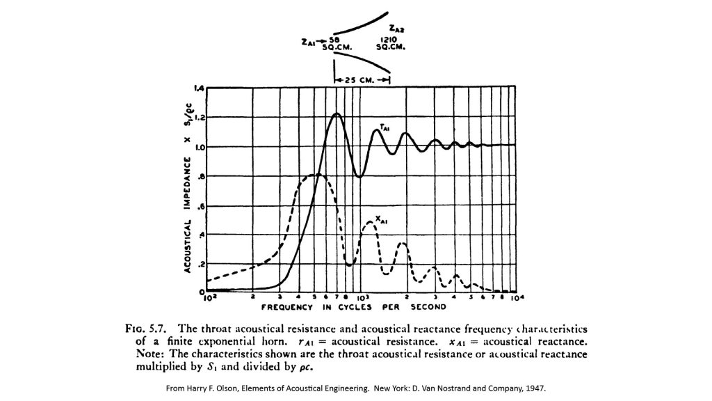
As mentioned above, I find the expressions for finite-horn throat impedance to be too complicated to be worth the trouble, so for this discussion I’m going to reproduce a chart from Olson [5] as an example of the predicted throat impedance of a exponential horn using the finite-horn approach:

As a comparison, the following figure shows the infinite-horn throat impedance for the same horn shape (which I calculated using equations I’ll introduce later in this post).

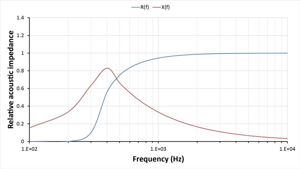
Obviously, the infinite-horn impedance plots of Figure 6 show no signs of the mouth resonance effects evident in the finite-horn plots previously shown in Figure 5. Otherwise, the infinite-horn impedance plots are reasonably close to the finite-horn plots, considering that they’re so much easier to calculate.

However, the classical finite-horn analysis approach of treating the mouth as a sharp high-pass cutoff filter doesn’t make sense in this example. That’s because, for this horn, the rule-of-thumb mouth cutoff frequency is about 600 Hz—but from the finite-horn plot of Figure 5, the relative throat resistance is still a a significant (albeit modest) 0.4 down to 400 Hz. So, assuming that this horn won’t work at all below the rule-of-thumb mouth cutoff frequency significantly underestimates its low-frequency capability.

For that reason, the approach I use in my own horn analyses is a modified version of the classical infinite-horn approach. I haven’t come across anyone else using this particular approach, and that could be because there’s something wrong with it…but, to me, it seems like a good balance between the simplicity of the classical infinite-horn approach and the fidelity of the finite-horn approach.

The modified Infinite-horn approach

According to the modified infinite-horn approach I use, the relative finite-horn throat resistance can be estimated by multiplying the mouth resistance by the infinite-horn throat resistance:

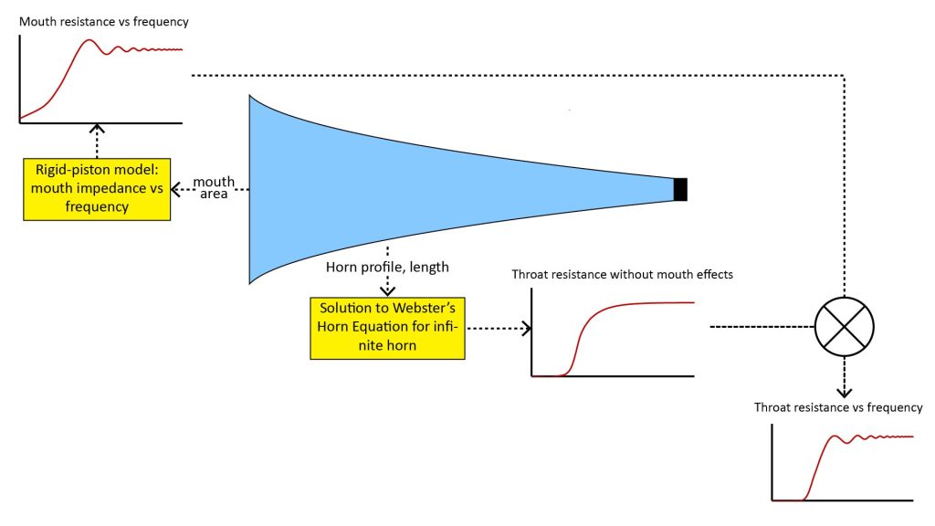
This avoids the complexity of the math for the finite-horn throat impedance, but does a better job of accounting for the mouth impedance than the simple rule-of-thumb mouth cutoff.

Figure 8 shows the infinite-horn throat resistance (the same curve as in Figure 6), the mouth resistance estimated using the rigid-piston model, and finally the estimated finite-horn throat resistance per the modified infinite-horn approach, obtained as a product of the other two curves

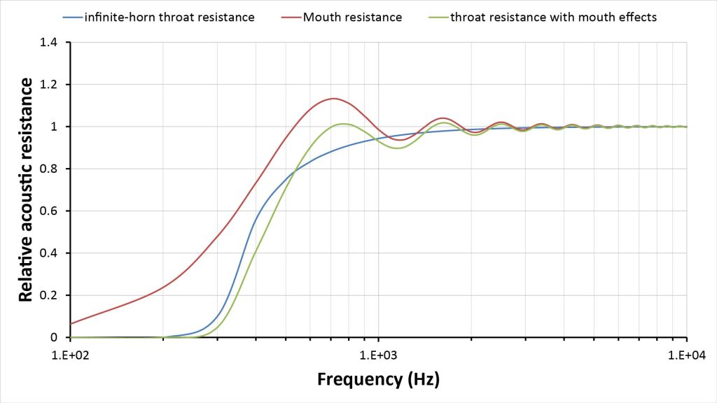
Note that this estimated finite-horn throat resistance is in better agreement with Olson’s finite-horn curve of Figure 5 than the traditional infinite-horn curve of Figure 6. The curve of Figure 8 does under-predict the amplitude of the ripples due to mouth resonance shown in Figure 5, but at least it indicates their presence.

The classical approach to analyzing what happens outside an APH

Now that we’ve discussed the impedance-transforming function of a horn, let’s talk about its directivity. Unlike impedance transformation, a horn’s directivity is determined by what happens outside the horn.

It seems intuitively obvious that putting a horn in front of an acoustic transducer (a microphone or speaker) should make the transducer more directional—and it does.

But there seems to be a lot of confusion about how a horn makes a transducer more directional. So, before I discuss the classical approach to predicting a horn’s directional characteristics, I think it’s worth talking about the physical basis for a horn’s directivity.

A horn’s directivity is mainly due to its mouth, not its profile

Someone who hasn’t studied horns might have the idea that it’s the profile of a horn that determines its directivity. According to this idea, the sides of the horn restrict the received or emitted sound to a particular range of angles that depends on the horn’s shape.

But if a horn’s profile were the only thing determining its directivity, then a narrow cylindrical pipe would behave like an “acoustic laser”, with much greater directivity than a flared horn with a wide mouth. Of course, this isn’t the case.

It turns out that, while a horn’s directivity is indeed influenced by its profile at higher frequencies, its low-frequency directivity is due to its mouth…and low-frequency directivity is often what limits the performance of a horn microphone.

The mouth of a horn provides directivity in the same way as other acoustically directive devices: via destructive interference of off-axis sound. Here’s a way to visualize how that works in a horn microphone:

• Sound reaching the horn causes the air in the horn’s mouth to vibrate.
• If the sound is arriving along the horn’s axis, then all of the air molecules across the mouth will vibrate in phase.
• But if the sound is arriving at an angle, there will be a phase gradient across the mouth, so that the air molecules won’t be vibrating in-phase. So, since the total sound power at the mouth is the vector sum of the sound powers of all the vibrating molecules, there will be less sound power available to reach the microphone.
• The larger the mouth, the greater the phase gradient for a given off-axis angle and wavelength, and thus the greater the directivity.
• Since the phase gradient depends on the wavelength, the directivity provided by any aperture of constant width is always frequency-dependent: it increases with increasing frequency.

All highly directional microphones exploit this principle of destructive interference across a relatively large sound-collecting aperture, and the same principle applies to any highly directional antenna used for either receiving or radiating electromagnetic waves.

The classical approach to estimating horn directivity

Up until the early 2000’s, the accepted way to predict the directional characteristics of any sound-collecting or sound-radiating aperture (such as the mouth of a horn) was to model it as a vibrating rigid piston mounted in an infinite baffle.

When applied to a horn speaker, such a model assumes, in effect, that the horn’s mouth is a large rigid speaker diaphragm with zero mass, and ignores the rest of the horn. Of course that’s not how a horn really works, so it’s obvious that the rigid-piston model has limited fidelity. However, it’s good enough for many purposes, and many excellent audio devices have been designed using rules-of-thumb based on the rigid-piston model.

Another advantage of the rigid-piston model is that the math was worked out almost a century ago and is relatively simple. See, for example, paragraph 2.10 of Olson [5].

So, the rigid-piston model for radiating apertures has been in vogue for many decades, not just for horn mouths but also for loudspeaker diaphragms. By the way, the rigid-piston model is equivalent to the uniformly-illuminated circular aperture model which is often used to analyze parabolic antennas and microphones; the math is the same.

But if the rigid-piston model has known limitations, why has it been used for so long? Because more accurate models aren’t amenable to closed-form analytic solutions, and therefore weren’t practical until computers became ubiquitous.

For example, while Morse and Ingard [7] suggested in section 7.2 of their 1968 textbook that greater fidelity could be obtained by modeling an acoustic aperture as a pulsating segment of a sphere (the spherical cap model), actual use of the spherical cap model didn’t become practical until decades later.

More recently, Morgans [4] shows how the spherical-cap model can be used to optimize the design of a horn speaker. Aarts and Janssen [8] verified the validity of the spherical-cap model by comparing predictions based on both the rigid-piston and spherical-cap models with measured data.

Unfortunately, while computer power is no longer an issue in using the spherical-cap model, the required numerical techniques are a little daunting for someone who isn’t already familiar with them.

That’s why I decided to stick with the tried-and-true rigid-piston model for my own horn analyses…but only if I could understand, and account for, the model’s limitations.

Using the rigid-piston model to predict a horn’s polar pattern and directivity

Figure 9 shows the standard equations to determine the polar pattern (the relative sound power versus off-axis angle) of a horn’s mouth under the rigid-piston assumption; the equations are applicable not just to horn mouths, but to any sound-collecting aperture. Notice the use of a Bessel function for the circular mouth equation; most spreadsheets and math analysis applications (such as MATLAB) include Bessel functions so it’s pretty easy to evaluate the formula.

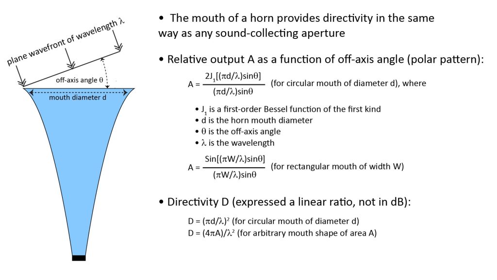
In addition to the polar pattern, Figure 9 shows the standard equations to approximate the mouth’s directivity, which (as for any directional microphone) is defined as the ratio of its on-axis response to its response averaged over all directions. As discussed in my post on long-range microphones, the directivity metric D is an extremely important metric in estimating the pick-up range of a directional microphone.

The limitations of the traditional rigid-piston model as applied to horns

The traditional approach to using the rigid-piston model to determine a horn’s directivity involves two implicit assumptions:

• that the acoustic wavefront at the horn’s mouth is planar, and
• that the amplitude and phase across the mouth are uniform.

Unfortunately, there are several phenomena in real horns that tend to reduce the validity of those assumptions:

• The wavefront at the mouth of a horn is never completely planar, with the degree of curvature depending on the shape of the horn..
• There can be resonances inside the horn that result in transverse modes in the wavefront. A transverse mode is a standing wave perpendicular to the horn’s axis, and will obviously cause a non-uniform amplitude/phase distribution across the mouth.
• Sound arriving at the mouth can experience a change in amplitude or phase as it travels to the microphone element at the throat—and depending on the shape of the horn, that change might be different for sounds arriving at different points in the mouth. This will have the same effect as a non-uniform amplitude/phase distribution across the mouth.

The latter two effects apply to the spherical-cap model as well as the rigid-piston model.

The extent of these effects all depend on the shape of the horn, and they all tend to make the horn’s mouth appear smaller (from a directivity perspective) as the frequency increases.

Referring again to Figure 9, the rigid-piston model says that horn directivity is proportional to the square of the ratio of the mouth diameter to the wavelength. Thus, the directivity predicted by the rigid-piston model increases with the square of the frequency. But, if the effective mouth size decreases with frequency, then the rigid-piston equation will obviously over-predict the actual directivity at higher frequencies.

Accounting for the limitations of the rigid-piston model

As far as I can determine from my literature review of this topic, there’s no simple method to accurately account for the limitations of the rigid-piston model in predicting horn directivity.

The only way to obtain accurate horn directivity predictions is to use numerical techniques such as Finite-Element Analysis (FEA) or the Boundary Element Method (BEM), but those are hardly simple techniques.

Fortunately, the relatively high accuracy achievable with such techniques isn’t necessary for many horn applications. And I believe that it’s possible to account for the limitations of the rigid-piston model sufficiently well to obtain useful directivity predictions for at least the two most useful horn shapes for microphone applications: the exponential horn and the conical horn. I’ll discuss why those are the most useful horn microphone profiles later in this post; for now, I’ll focus on how I estimate their directivity.

My approach is based on review of horn polar patterns and directivity data (from either measurements or numerical modeling) reported in the literature. There isn’t a lot of such data, but it’s enough to get a better idea of how real horns work than by just relying on the rigid-piston model. For copyright reasons, I’ll use data from Olson [5], which is now in the public domain, to illustrate my approach.

What Olson says about horn directivity versus frequency

Olson observed that a horn speaker’s polar pattern doesn’t get sharper with frequency in exactly the same way as predicted by the rigid-piston model. Here’s what he says, in section 2.14, about this effect:

“The mouth of the horn plays a major role in determining the directional characteristics in the range where the wavelength is greater than the mouth diameter. The flare is the major factor in determining the directional characteristics in the range where the wavelength is less than the mouth diameter.“

Olson provided data for both exponential and conical horns to illustrate this effect. Olson doesn’t say if these were measured data or calculated data (or, if the latter, how they were calculated). However, by the time the second edition of his Elements of Acoustical Engineering was published in 1947, Olson had been director of acoustical research at RCA laboratories (which was a leading manufacturer of horn speakers) for more than a decade, so I have no hesitation in accepting his data.

Exponential horn directivity

In an exponential horn, the cross-sectional area increases exponentially with distance from the throat. The exponential horn is by far the most common type of horn in speaker applications and is also very useful in microphone applications; we’ll discuss why later.

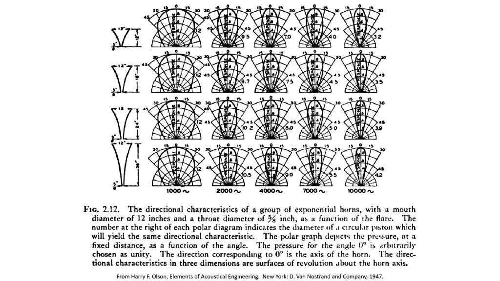
In section 2.14 A, Olson [5] says this about the directional characteristics of exponential horns:

“It will be seen that up to the frequency at which the wavelength becomes comparable to the mouth diameter, the directional characteristics are practically the same as those of a piston of the size of the mouth. Above this frequency the directional characteristics are practically independent of the mouth size and appear to be governed primarily by the flare“.

To illustrate this, Olson showed the polar pattern and effective mouth diameter for four different exponential horn flare constants at five different frequencies, these data are reproduced here as Figure 10:

Another way to look at Olson’s data is to plot the relative mouth diameter (the ratio of the effective to actual diameters) versus the ratio of the actual diameter to the wavelength, as I’ve done below:

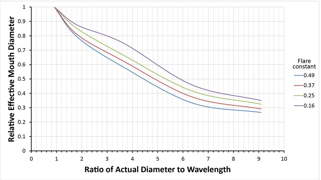
We can take this a step further: since we know that the directivity of a circular aperture is proportional to the square of its diameter, we can take the square of the relative effective mouth diameters of Figure 11 to obtain a directivity derating factor for exponential horns:

We can use these directivity derating factors to estimate the frequency-dependent directivity of any exponential horn that has a flare constant similar to those examined by Olson. To do that, we just multiply the directivity derating factor at the desired frequency by the rigid-piston directivity given by the equation of Figure 9.

To make this process easier, I fit exponential curves to the curves of Figure 12 to eliminate the need for interpolation; more on that later.

Conical horn directivity

In a conical horn, the cross-section width increases linearly with distance from the throat, so the cross-section area increases with the square of the distance from the throat. Conical horns are never used in speaker applications but they can be useful for microphones; we’ll discuss why later.

In section 2.14 B, Olson [5] says this about the directivity of conical horns:

“At lower frequencies the directional pattern is approximately the same as that of a piston of the same size as the mouth. The directional pattern becomes sharper with an increase of the frequency. However, at the higher frequencies where the diameter of the mouth is several wavelengths, the pattern becomes broader as would be expected from a spherical surface source”.

Olson illustrates this point with a figure, reproduced here as Figure 13:

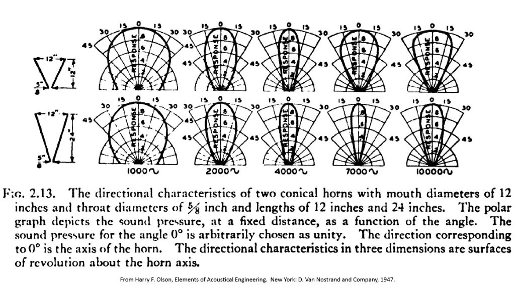
Notice that the polar patterns at the highest frequency (10 kHz) are shaped very much like the horn cross-sections (shown to the left of the figure). In other words, the beamwidths at the highest frequency are comparable to the horn angles (which are 51 degrees for the shorter horn and 27 degrees for the longer horn).

In fact, there’s an old rule-of-thumb that says that, above a certain frequency, the beamwidth of a conical horn is constant and approximately equal to the horn angle. This is based on the fact that a conical horn is actually a section of a sphere, so the wavefront inside a conical horn speaker expands as it travels through the horn just as it would in free space. Therefore, neglecting diffraction from the edges of the mouth, the wavefront should continue expanding at the same rate after leaving the mouth, forming a conical beam of the same beamwidth as the horn angle.

The bigger the horn angle, the more significant the wavefront curvature at the mouth, and the lower the frequency at which the mouth stops acting like a rigid piston and the horn begins to produce a conical beam.

We can see this effect more clearly by comparing Olson’s conical horn beamwidths to the beamwidth predicted by the rigid-piston model of Figure 9. I show such a comparison in Figure 14, which plots the -3 dB beamwidths of Olson’s two conical horns and a rigid piston as a function of d/λ (the ratio of mouth/piston diameter to wavelength):

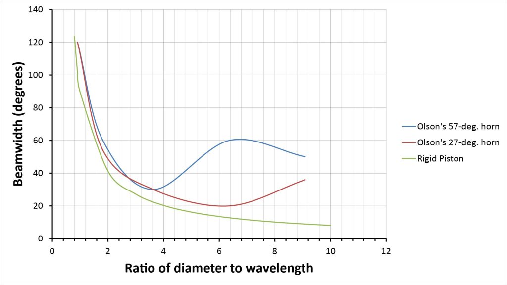
Olson’s conical horn beamwidths track the rigid-piston beamwidth downward with increasing d/λ ratio (and, hence, with increasing frequency), but then bottom out and start increasing again at a d/λ ratio that depends on the horn angle (specifically a d/λ ratio of about 3.6 for the 51-degree horn, and a ratio of about 6.4 for the 27-degree horn). As the frequency increases still further, the horn beamwidths peak and then begin to decrease again (although Olson’s data doesn’t extend high enough in frequency to reach this point for the 27-degree horn). Eventually, the beamwidths stabilize to values that are approximately equal to the horn angles, and you can see that the 57-degree horn has almost reached this point at a d/λ ratio of 9 (which corresponds to about 10 kHz).

Thus, a conical horn has the beamwidth of a rigid-piston at low d/λ ratios, but a beamwidth equal to the horn angle at high d/λ ratios. The d/λ ratio at which the beamwidth transitions from rigid-piston to horn angle depends on both the horn angle and the mouth diameter: a horn with a small mouth diameter and a small horn angle will maintain the beamwidth of a rigid piston up to a high frequency, while a horn with a large mouth diameter and a large horn angle will transition to the horn-angle beamwidth at a lower frequency.

These observations suggest that, if we’re willing to accept some inaccuracy at the transition point, we can approximate the beamwidth of a conical horn at any d/λ ratio as the greater of the rigid-piston beamwidth and the horn angle. Figure 15 shows such an approximation overlaid on the curves previously shown in Figure 14:

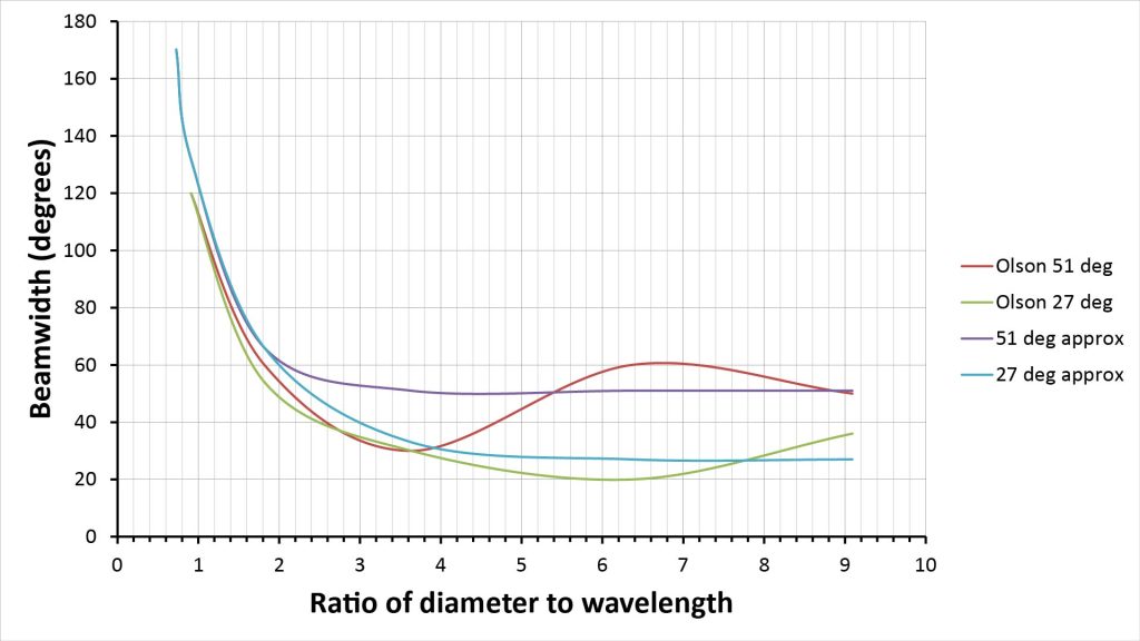
There’s some inaccuracy before and after the point at which the horns transition from rigid-piston to conical-beam behavior, but the estimate is certainly more accurate than either the rigid-piston or horn-angle alone.

Figure 15 suggests a very simple way to estimate the directivity of a conical horn: because directivity is inversely proportional to the square of the beamwidth, the directivity of a conical horn at a given wavelength can be approximated as the lesser of the rigid-piston directivity and the conical-beam directivity. There will be some error in the estimated directivity around the d/λ ratio at which the behavior transitions from rigid-piston to conical-beam, but it should still be more than accurate enough for most design applications.

Fortunately, the equation for conical-beam directivity is quite simple (see Wikipedia, “Directivity”), as we’ll discuss later.

Accounting for Transducer directivity

So far, our directivity discussion has been limited to the horn itself, and we’ve seen that horn directivity can remain constant (for a conical horn) or even decrease (for an exponential horn) at high frequencies.

However, the transducer used with the horn (the microphone element in a horn microphone, or the compression driver in a horn speaker) will also have its own directivity. Per the rigid-piston model, this directivity will be determined by the diameter of the transducer’s diaphragm (which is typically but not necessarily equal to the horn’s throat diameter).

Depending on the transducer diameter, its directivity could be so high at higher frequencies that the transducer’s polar pattern doesn’t even touch the walls of the horn. In this case, the transducer directivity is greater than that of the horn and determines the overall directivity.

Therefore, we can account for the transducer directivity by estimating the overall directivity as the greater of the horn directivity and the transducer directivity.

Adapting APH speaker theory to horn microphones

All of the APH theory we’ve discussed so far comes from the field of horn speakers. However, most things in physics obey a reciprocity law, and horns are no exception: horn speaker theory is directly applicable to horn microphones.

However, there is one horn performance metric that usually isn’t analyzed for speakers, but is potentially important for microphones: horn gain.

Horn gain is the increase in sensitivity provided by the horn

As mentioned in the introduction to this post, the APH in a horn microphone amplifies the acoustic pressure at the microphone element. The pressure amplification factor is the horn gain, and it’s equal to the acoustic resistance of the throat divided by the acoustic resistance of the mouth.

This same horn gain is also the gain in efficiency provided by the horn in a horn speaker. However, the absolute gain is not usually calculated in horn speaker design; instead, the focus is on the flatness of the throat impedance versus frequency curve.

In contrast, calculating the absolute gain is potentially important in horn microphone design, for two reasons:

• It influences the Signal-to-Interference-plus-Noise Ratio (SINR) at the output of the microphone, especially in situations in which there is relatively little ambient noise.
• It determines the required maximum-SPL rating of the microphone element. If the horn gain is very high, then the SPL at the microphone can easily reach levels that cause clipping or even permanent damage.

Estimating APH gain

Fortunately, estimating the pressure gain provided by an APH is trivial: it’s just the ratio of the mouth area to the throat area. Of course, the full measure of this gain will occur only when the mouth and throat impedances are completely resistive, so the gain is frequency-dependent. It can be thought of as a multiplier on the relative horn efficiency discussed in the section on acoustic-impedance transformation.

Horn profiles for APH microphones

Now that we’ve discussed some of the basic horn theory, we can get into the pros and cons of various horn profiles for APH microphone applications.

As I’ve already mentioned, I believe that the exponential and conical horn profiles are the most useful for APH microphones. But before I attempt to justify that assertion, let’s discuss horn profiles in general and the criteria we might use to assess them for microphone applications.

Horn profiles used in speaker applications

A horn’s profile defines the relationship between its cross-sectional area and axial distance from its throat. In an exponential horn, the cross-sectional area increases exponentially with distance from the throat, while in a conical horn, the cross-sectional area increases as the square of the distance from the throat.

While the exponential profile is the most widely-used profile in speaker applications, many other profiles are also used in speakers. One reason for this wide variety of horn speaker profiles is that horn speakers must balance three conflicting design requirements:

• High efficiency at low frequencies.
• Avoidance of ripples in the frequency response.
• Avoidance of excessive directivity at high frequencies.

These design constraints result in inevitable compromises, and the large variety in horn shapes allow speaker designers to minimize the impact of those compromises for a given application.

Maximizing low-frequency efficiency and flatness of frequency response

In the early days of horn speaker design, amplifier power was very expensive, so low-frequency efficiency was of paramount importance. As we’ve already discussed, a horn’s efficiency is proportional to the resistive component of its throat impedance, so the resistance-versus-frequency curve was the most important metric for early horn designers. The classic example is this famous chart from Olson [5], which has been widely reproduced since:

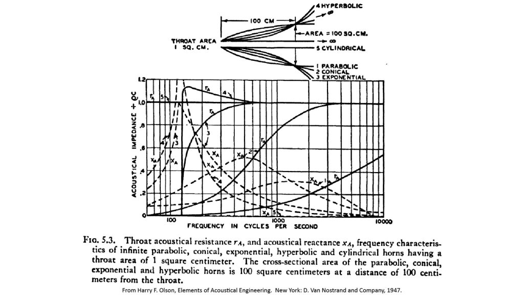
Note that these curves are for infinite horns, so they don’t include the ripples caused by the mouth impedance.

We can see from the curves of Figure 16 that the horn profiles represent a trade-off between the -3 dB low-frequency cutoff frequency (for given horn size) and the smoothness of the frequency response:

• The parabolic profile (curve 1) has the smoothest response, but the -3 dB cutoff frequency is so high (about 8 kHz) that a speaker using the parabolic profile would have to be even larger than the already-considerable 40-inch length of the horns of Figure 16 to be usable in audio applications.
• At the other extreme, the hyperbolic profile (curve 4) has the lowest -3 dB cutoff frequency, but the reactance (dashed) curve peaks sharply at cutoff, causing standing waves and resonances which in turn cause audible artifacts.
• The exponential profile (curve 1) seems to offer the best tradeoff: the -3 dB cutoff frequency is almost as low as that of the hyperbolic profile, but resistance curve is smooth and the reactance peak is more constrained. This is why the exponential horn has been so widely used in speaker applications.
• The conical profile’s -3 dB cutoff is much higher than that of the exponential horn (700 Hz versus 200 Hz for the horns of Figure 16), which is why it is never used in speaker applications. On the other hand, the cutoff of the conical horn is gradual and it has a usable response below the -3 dB frequency, whereas the exponential horn doesn’t. The conical horn also has another important advantage, which we’ll discuss next.

Controlling directivity

The advent of solid-state amplifiers in the 1960’s reduced the importance of efficiency as the driving requirement in speaker design. High efficiency was still considered a key advantage of horn speakers, but because amplifier power was no longer an issue, horn designers could begin to confront one of the disadvantages of high-efficiency horns: beaming, or excessive directivity, at high frequencies.

Very high directivity is undesirable in a speaker because it reduces the size of the listening “sweet spot”. Directivity that changes with frequency is also undesirable, because it distorts the frequency response at slight off-axis angles.

A horn speaker exhibits both of these effects. And it turns out that simple horn profiles that are best from an efficiency standpoint are the worst from a directivity standpoint.

Conversely, the conical horn profile (which is never used in speaker applications because of its poor low-frequency efficiency) is generally considered to have the best directivity characteristics for a speaker. That’s because it theoretically has a constant high-frequency directivity that’s less than that of more efficient horn profiles.

So, the holy grail in horn speaker design since the mid-1970’s has been a profile that offers the efficiency of an exponential profile with the near-constant directivity of a conical profile. Horns that attempt to achieve this are called constant-directivity horns, even though their directivity is apparently less constant than that of conical horns.

Horn microphones present different challenges

For horn microphones, the relative importance of efficiency vs directivity is the opposite of the situation with speakers:

• It’s much easier to compensate for poor low-frequency response in a microphone than in a speaker (amplifier power and transducer power-handling capacity are non-issues with microphones).
• The main motivation for coupling a horn to a microphone is for long-range pickup. So, unlike horn speakers, high directivity is generally an advantage for microphones, and directivity that changes with frequency isn’t a problem because the microphone will generally be pointed directly at the source. On the other hand, extremely high directivity can be a problem because it makes microphone aiming more difficult.

For these reasons, the conical horn—which is never used in horn speakers—can be quite useful for medium-range microphone applications. Its smooth low-frequency roll-off can be electronically equalized to extend the response to at least an octave or two below the -3 dB frequency, and its near-constant directivity ensures good high-frequency response at slight off-axis angles (which facilitates microphone aiming). Plus, the conical horn is by far the easiest and cheapest horn to fabricate.

The exponential profile is also extremely useful in horn microphones, and is preferable to the conical profile at longer ranges where its greater high-frequency directivity is a major advantage. Exponential horns are also less expensive than all other horn types (except conical horns) due to their ubiquity in speaker applications.

And that’s why I believe the conical and exponential profiles are the best horn profiles for APH microphone applications.

The key equations for conical and exponential APH design

Now that I’ve discussed the theory underlying horn speakers, I’m going to summarize the key equations I use to design or analyze APH microphones using the conical and exponential horn profiles. These are shown in Figures 17 and 18 below, and if you’ve read the preceding material, they should seem pretty straightforward. However, there are few points that merit further discussion.

For both profiles, the equations are grouped into three categories, corresponding to the three attributes that are most important in horn microphone design:

• Directivity
• Frequency response
• Gain

Not surprisingly, design of APH microphones using conical and exponential profiles involves different trades between these three attributes.

The key conical APH design equations

Figure 17 summarizes my approach to designing or analyzing APH microphones using the conical horn profile.

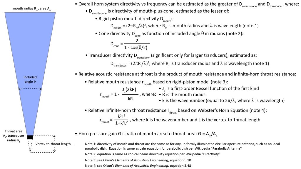
Conical APH directivity estimation

As already mentioned, I estimate conical horn directivity as the greater of the mouth/cone directivity and the transducer directivity:

• The transducer directivity will come into play at audible frequencies only for horns that use a transducer (or an array of transducers) with a diameter of more than a few inches. Transducer directivity can be estimated easily using the circular aperture directivity equation shown.
• The mouth/cone directivity is estimated as the lesser of the mouth directivity (obtained using the circular-aperture equation) and the cone angle.

Conical APH Frequency response estimation

As I’ve already described, an APH’s relative-throat-resistance-versus-frequency curve is a good proxy for its frequency response. And per my modified infinite-horn approach, I estimate the relative throat resistance of a finite horn as the product of the mouth resistance and the infinite-horn throat resistance.

The mouth resistance equation for a conical horn (which requires evaluation of a first-order Bessel function of the first kind, which is included in most spreadsheet programs) is the same as for the mouth of an exponential horn (or any circular aperture).

However, the infinite-horn throat resistance equation for a conical horn is different from that of an exponential horn. Not only is the form different, but the equation is a bit counter-intuitive because it doesn’t directly depend on the length of the horn. Instead, it depends on the horn’s vertex-to-throat distance, which is the “missing” part of the cone behind the throat. The smaller this distance, the poorer the horn’s low-frequency response. We’ll discuss the implications of this shortly.

Conical APH pressure gain

As with all APH’s, the pressure gain of a conical APH is equal to the ratio of the mouth to throat areas. We’ll discuss the implications of pressure gain later.

Key conical APH design trades

As noted above, a conical APH’s frequency response depends on the vertex-to-throat length (the “missing” part of the horn). This vertex-to-throat length varies with the throat diameter and the horn angle, so we can improve a conical APH’s frequency response by either reducing horn angle or increasing the throat diameter:

• We can increase the vertex-to-throat distance by decreasing the horn angle. But this will also reduce the mouth diameter unless we also increase the horn length. Reducing the mouth diameter is generally a bad trade because it will shift the mouth resistance curve to higher frequencies (potentially offsetting any improvement in low-frequency response from reducing the horn angle), while also reducing directivity and gain. So, if we want to improve the low-frequency response by reducing the horn angle, we generally also want to increase the horn length. All APH profiles exhibit a similar relationship between horn length and low-frequency response.
• Alternatively, we can increase the vertex-to-throat distance by increasing the throat diameter (which will also shorten the horn’s actual length by the same amount, if we keep the same horn angle). But since the horn gain is equal to the ratio of the mouth area to the throat area, increasing the throat diameter will also reduce the horn gain. Thus, for a conical APH, there is a trade between low-frequency response and gain: if we want better low-frequency reponse but we want to keep the same horn angle, we have to accept reduced horn gain. A similar trade also applies to the exponential horn.

The conical horn also offers an interesting trade in directivity. Increasing the mouth diameter increases the low-frequency directivity, but unless the horn length is also increased, the horn angle will increase…which will reduce the high-frequency directivity. So, for a given horn length, varying the mouth diameter trades between low-frequency directivity and high-frequency directivity (besides also affecting the frequency response via the mouth impedance).

The key exponential APH design equations

Figure 18 summarizes my approach to designing or analyzing APH microphones using the exponential horn profile.

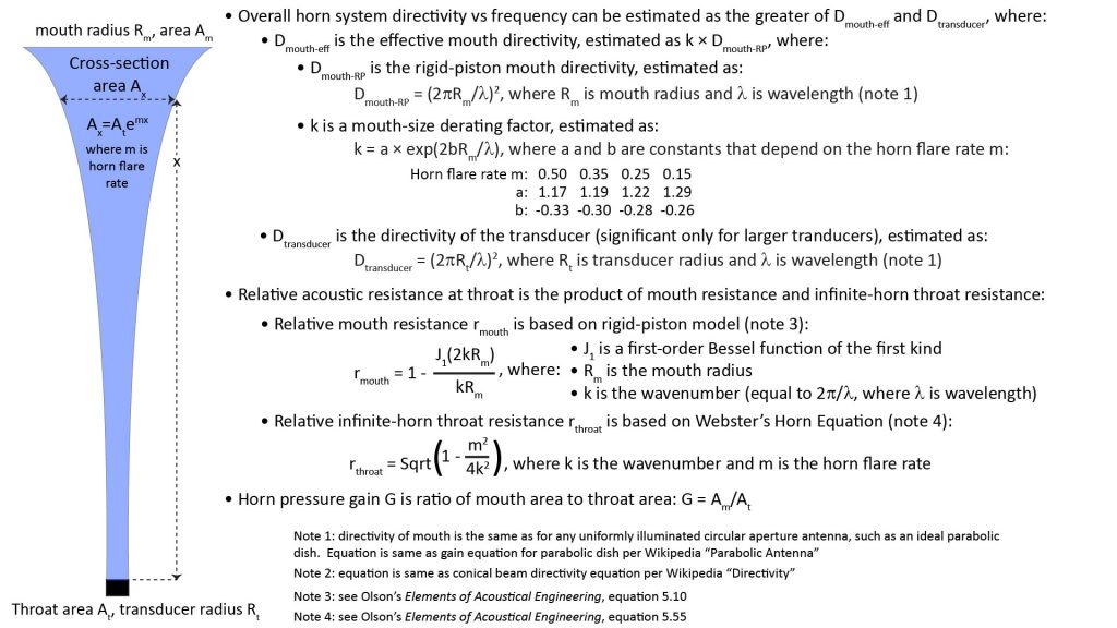
Exponential APH directivity estimation

As with the conical horn, I estimate the directivity of an exponential horn as the greater of the mouth/cone directivity and the transducer directivity:

• The transducer directivity is estimated in exactly the same way as for a conical horn: via the standard circular-aperture directivity equation. As with the conical horn, transducer directivity will come into play at audible frequencies only for horns that use a transducer (or an array of transducers) with a diameter of more than a few inches.
• However, the mouth/cone directivity of an exponential horn is estimated differently than for a conical horn. For the exponential horn, I estimate directivity using the standard circular-aperture directivity equation, but I multiply that directivity by a derating factor that accounts for the fact that an exponential horn’s effective mouth diameter decreases with frequency. As you can see from Figure 18, the derating factor I use is an exponential function that requires two parameters that depend on the horn’s flare constant. The figure shows a table of parameter values for four flare constants; I just use the parameter values for the flare constant that’s closest to that of the horn I’m analyzing (this is just an approximation, so some error in the parameter values is fine).

Exponential APH frequency response estimation

The only difference between my approaches for estimating exponential and conical APH frequency response is in the form of the infinite-horn throat-resistance equation.

Whereas the horn design parameter that determines a conical horn’s infinite-horn throat resistance is the vertex-to-throat distance, the design parameter that determines an exponential horn’s throat resistance is the exponential flare constant.

Also, you can see that the exponential horn’s infinite-horn throat resistance will drop to zero when m²/4k² = 1, where m is the flare constant and k is the wavenumber. The frequency at which this occurs is called the throat cutoff, and the conical horn doesn’t have such a sharp cutoff.

However, in a finite exponential horn, the throat resistance doesn’t really drop to zero at the cutoff frequency; it’s greatly attenuated, but non-zero.

Exponential APH pressure gain

The pressure gain of an exponential APH is found exactly the same way as for a conical APH: as the ratio of the mouth to throat areas.

Key exponential APH design trades

Although the equations are different, the design trades for an exponential horn are very similar to those for a conical horn:

• As with the conical profile, the exponential profile offers a trade between pressure gain and frequency response. This is because the exponential horn’s infinite-horn throat resistance depends on the flare constant, which relates the throat diameter to the mouth diameter and horn length. For the same mouth diameter and horn length, a smaller flare constant (which improves the low-frequency response) implies a larger throat, which in turn results in a smaller pressure gain.
• As with the conical profile, the exponential profile also offers a trade between horn size and frequency response: the larger the horn, the better the low-frequency response.
• As with the conical profile, the exponential profile also offers a trade between low-frequency and high-frequency directivity: increasing the mouth diameter increases the low-frequency directivity, but unless the horn length is also increased, the flare constant will increase…which will reduce the high-frequency directivity by increasing the directivity derating factor. So, for a given horn length, varying the mouth diameter trades between low-frequency directivity and high-frequency directivity (besides also affecting the frequency response via the mouth impedance).

Comparing conical and exponential horns

In this section I’m going to use the equations of Figures 17 and 18 to compare three pairs of conical and exponential horns. The objective is partly to illustrate how the equations can be used, and partly to illustrate the trade-offs between the two horn profiles with some specific examples.

The cross-sections of the horns I’ll be comparing are depicted in Figure 19:

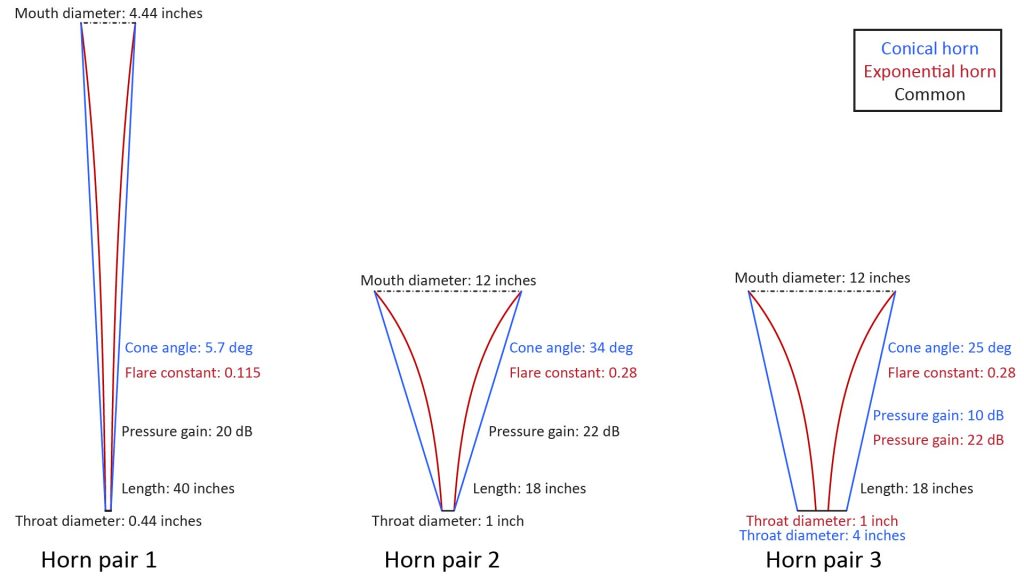
Pair 1: Olson’s infinite conical and exponential horns

The first pair of horns in Figure 19 have the same conical and exponential profiles Olson used in his famous infinite-horn impedance chart (reproduced above as Figure 16). Many authors cite this chart when dismissing the conical horn for practical applications, because it shows that the conical horn has a much higher throat cutoff than the exponential horn.

However, Olson’s chart is for infinite horns, which means that it doesn’t include the effects of mouth impedance (Olson [5] also presents impedance curves for some exemplar finite conical and exponential horns, but the profiles aren’t the same as those in his famous infinite-horn impedance chart).

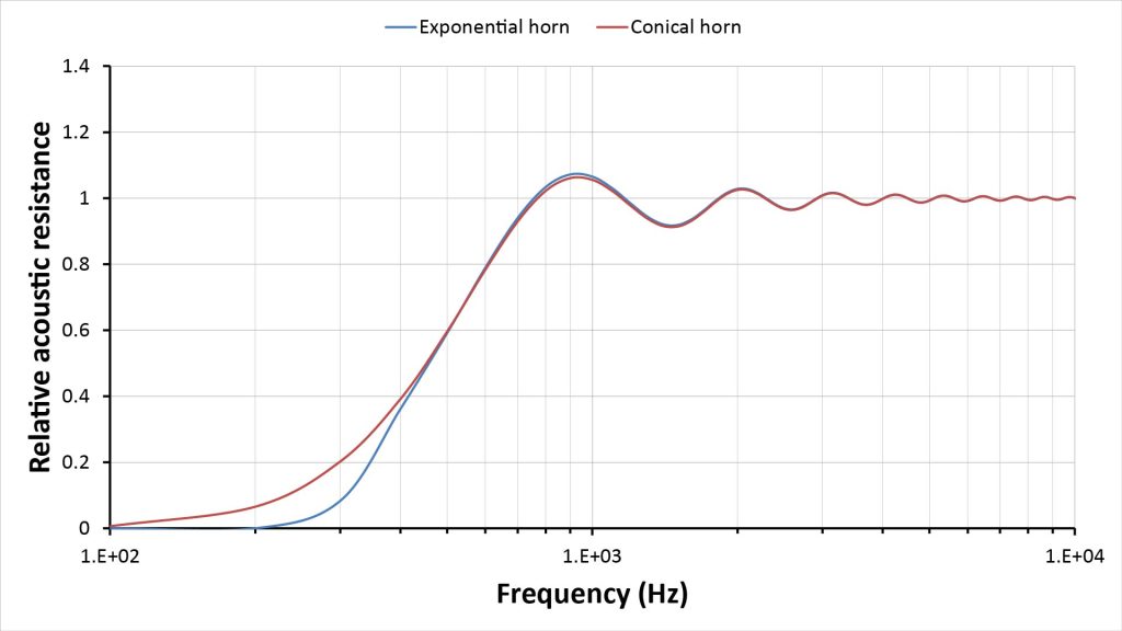
If we’re willing to accept approximate results, we can use my modified infinite-horn approach (previously illustrated in Figure 7, and summarized in Figures 17 and 18) to comprehend the effects of mouth impedance. This yields the following throat-resistance curves for the same conical and exponential horns of Olson’s infinite-horn chart:

Notice that the exponential horn’s huge advantage in low-frequency response that was evident in Figure 16 has evaporated. This is because the actual low-frequency cutoff for both of these horns is limited by the mouth, not the throat…and the mouth is the same size for both horns.

This is an extreme example, because the hypothetical horns modeled in Olson’s famous infinite-horn chart have extremely small mouths. The small mouths limit not only the low-frequency response (especially for the exponential horn), but also the low-frequency directivity.

Still, Figure 20 shows that, when mouth impedance is taken into account, the frequency-response gap between conical and exponential horns isn’t always as huge as might be expected.

How about directivity? Well, I’m not going to show directivity projections for these particular horns, because the exponential horn’s flare rate and the conical horn’s cone angle are so small that the directivity estimation approaches of Figures 17 and 18 might not be valid.

Now let’s look at some more practical horns.

Pair 2: practical conical and exponential horns of same size

A practical horn profile for an APH microphone will have a larger mouth than the horns we just examined…not just for improved low-frequency response (due to the greater mouth cutoff frequency), but also for enhanced directivity.

So the horns of pair 2 of Figure 19 have larger mouths (but shorter lengths) than the horns in the previous comparison.

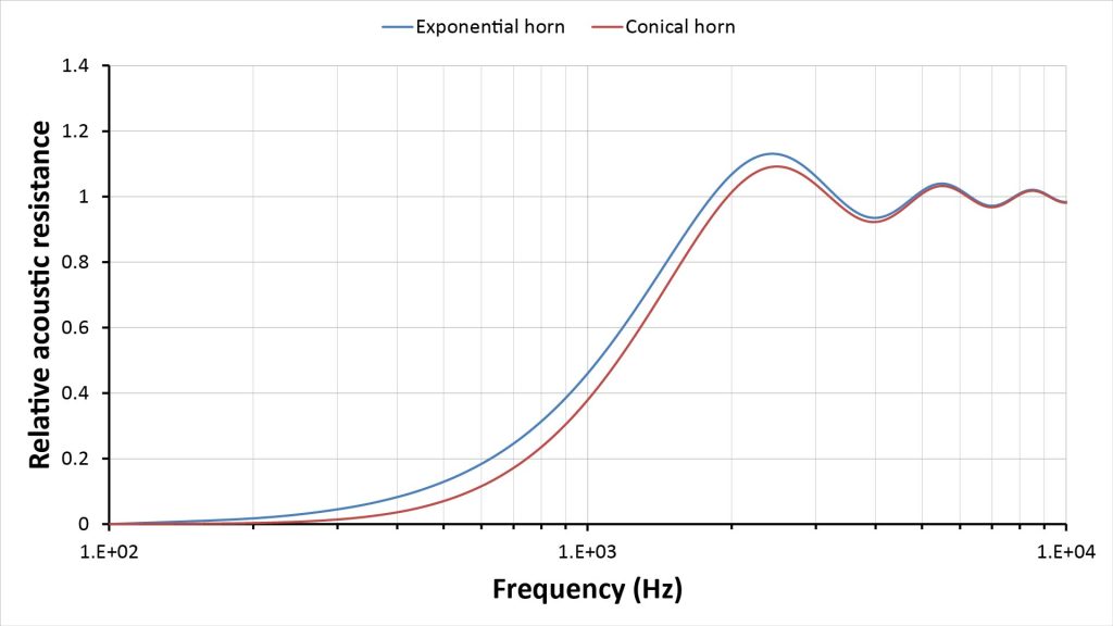
Figure 21 shows the throat impedance versus frequency curves for these two horns obtained using the equations of Figures 17 and 18:

With the much larger mouths of these horns, the mouth resistance no longer limits the throat resistance, so (as we would expect) the exponential horn has much better low-frequency response: it has a -3 dB cutoff of about 450 Hz, while the conical horn has a -3 dB cutoff of about 1300 Hz.

However, the conical horn’s response rolls-off more smoothly, and if we apply a modest 10 dB of electronic equalization we can extend the response down to about 500 Hz. However, that 10 dB of low-frequency gain will also boost the ambient noise and microphone self-noise at those frequencies.

So the exponential horn is definitely better from a bandwidth standpoint, but the conical horn is certainly usable.

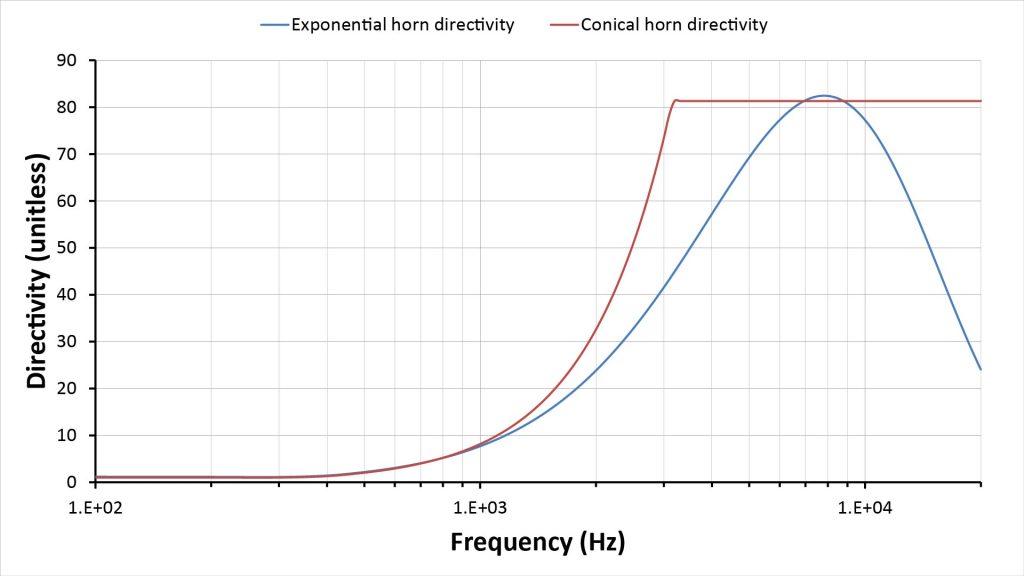
Now let’s consider directivity. Figure 22 shows the predicted directivity of pair 1 using the equations of Figures 17 and 18:

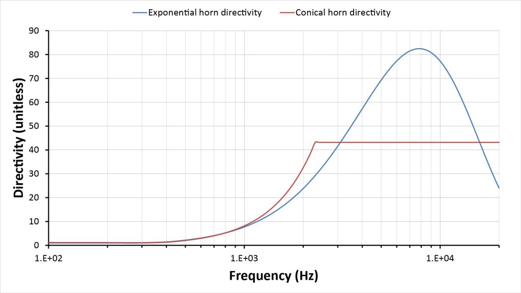
As we would expect (because the mouth diameters are the same), both horns have the same modest low-frequency directivity, but the directivity curves begin to diverge around 2 kHz. The conical horn has a flat directivity of 43 (or 16 dB) above that frequency, while the exponential horn’s directivity peaks at about 81 (or 19 dB) at 9 kHz.

So the exponential horn offers 3 dB greater peak directivity, but the directivity isn’t flat at the higher frequencies as it is for the conical horn. One issue with frequency-dependent directivity is that it affects the frequency response at slight off-axis angles. A conical horn has a wider sweet-spot over which the high-frequency response is nearly flat, which can be a significant advantage at shorter ranges.

Finally, let’s consider the pressure gain. The gain is determined completely by the mouth and throat areas, so it’s the same for both horns (144, or 22 dB, as shown in Figure 19. Gain is great as long as there’s no risk of over-driving the microphone element. If we assume that the microphone element can handle 120 dB SPL without distortion, then we can use these horns to pick-up a target signal of up to 98 dB SPL without distortion. If we assume a flat 16 dB of directivity, then the 22 dB gain means we can also operate the horns in up to 114 dB SPL of isotropic ambient noise without distortion. Both these figures (a maximum target signal level of 98 dB SPL and a maximum ambient noise level of 114 dB SPL) are more than ample for typical scenarios, so we can conclude that the risk of over-driving the microphone element is low.

So which horn is better? The exponential horn has a wider frequency response and slightly higher peak directivity, but the conical horn has a smoother response and flat high-frequency directivity. The exponential is probably better at longer ranges (due to the slightly higher peak directivity and the reduced need for low-frequency equalization), but the conical horn might be better at medium ranges (due to the wider sweet-spot over which the high-frequency response is flat).

Pair 3: conical horn with improved low-frequency response vs exponential horn

The conical horn in our pair 2 comparison above needs electronic equalization to reach down to 500 Hz. Let’s see what happens if we trade some pressure gain for improved low-frequency response.

Pair 3 of Figure 19 includes such a conical horn, along with the same exponential horn of pair 2. This new pair 3 conical horn has the same length and mouth diameter as the pair 2 conical horn, but the throat diameter has been increased from 1 inch to 4 inches. Increasing the throat diameter has three effects:

• It reduces the cone angle (specifically from 34 degrees to 25 degrees), which should increase the high-frequency directivity.
• It reduces the pressure gain (specifically from 22 dB to 10 dB).
• Finally, it increases the vertex-to-throat distance, which should improve the low-frequency response.

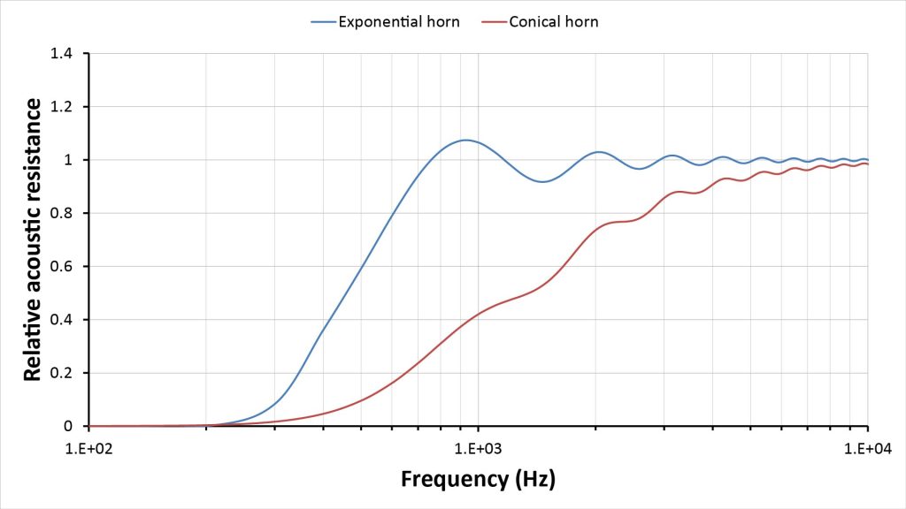
Figure 23 shows the predicted frequency response, along with that of the previous (pair 2) exponential horn:

The conical horn’s -3 dB low-frequency cutoff is now almost exactly the same as that of the exponential horn (450 Hz)…and with 10 dB of equalization, it could be extended even lower to around 250 Hz. The exponential horn’s cutoff is more abrupt and less amenable through extension via electronic equalization.

As previously mentioned, increasing the throat diameter also reduces the horn angle, which should improve the directivity. We can see the results in Figure 24, which shows directivity projections for both horns:

Both horns now have the same peak directivity of about 81 (19 dB), but the conical horn retains the advantage of a flat high-frequency directivity.

Of course, the loss in gain (from 22 dB down to 10 dB) could be a disadvantage in some applications. My post on long-range directional microphones discusses the impact of gain and directivity in detail, but the upshot is that directivity is more important than on-axis gain in most long-range applications, so the conical horn of pair 3 is likely preferable to the exponential horn in many applications.

Conical and exponential horns are the most practical profiles for APH microphones

Earlier in this post I stated that the conical and exponential horns are the most useful profiles for use in APH microphones. Hopefully I’ve demonstrated that the conical profile (which is generally dismissed as being unusable for speaker applications) is potentially very useful in microphone applications, but I haven’t really addressed profiles other than the conical and exponential profiles.

Part of the reason is that other horn profiles used in speaker applications (such as the hyperbolic, the Tractrix, and others) aren’t as amenable to simple analysis, which alone makes them less appealing (to me, at least).

Further, horns with these other profiles are harder to find in ready-made form than conical and exponential horns, and are much more difficult to fabricate from scratch than conical horns.

And in exchange for these disadvantages, these other horn profiles don’t offer any compelling advantages in the context of APH microphones. Constant-directivity horns do provide flatter directivity than exponential horns with better low-frequency response than conical horns, but these advantages are much less significant for microphones than for speakers.

A closer look at Acoustic Velocity Horn (AVH) microphones

Now let’s switch gears to to take a closer look at AVH microphones. I’ve already summarized the differences between APHs and AVHs in table 1 earlier in this post, but here’s another, even briefer, summary to set the stage for the following discussion:

• An Acoustic Velocity Horn (AVH) microphone uses a pressure gradient microphone (not a pressure microphone) mounted in the open (not sealed) throat of a horn, and provides amplification of the volume velocity (not the pressure) arriving at the horn’s mouth.
• Unlike an APH, an AVH does not act like a high-pass filter; instead it maintains its velocity gain down to virtually zero frequency, regardless of horn size. So, even a small AVH can provide excellent low-frequency response.
• One the other hand, the usable high frequency response of an AVH is potentially limited by its fundamental resonant frequency, which could significantly reduce the scope of potential AVH applications. I’ll explain why I use the word “potentially” shortly.

Another difference is that AVH microphones are even rarer than APH microphones. In fact, I’m not aware of any actual usage of AVH microphones, whereas APH microphones were relatively widely used at one point (for example, all early telephone mouthpieces used APHs).

There is also much less information on AVH theory and design. All of the available information seems to be contained in four relatively recent papers (the earliest having been published in 2011), which I’ve listed in the References at the end of this post. Those papers are quite informative, but there are two aspects of AVH operation that still aren’t clear (at least to me):

• As I’ve mentioned, resonance potentially limits the usable bandwidth of an AVH. Three of the four papers I’ve reviewed imply that AVHs might not be usable above the fundamental resonant frequency, while the fourth suggests that wideband operation is feasible.
• On a related subject, none of the papers discusses the directivity of AVHs at frequencies above the fundamental resonant frequency. I suspect that AVHs behave like APHs when it comes to high frequency directivity…but they might not.

I plan to resolve these issues to my satisfaction by actually building and testing some AVHs. Until then, the information herein on wideband operation of AVHs should be considered speculative.

Resonance in AVH microphones

All horns resonate at a fundamental frequency that depends on the horn size and shape, and whether the throat is sealed or open:

• If the throat is sealed (as in an APH), then the fundamental resonance is a standing wave with a node (an amplitude minimum) at the horn’s open mouth, and an anti-node (a pressure maximum) at the horn’s sealed throat. Thus, the wavelength of the fundamental resonance in an APH is equal to twice the effective length of the horn. I use the term “effective length” because the actual resonant frequency depends on the throat and mouth radii as well as the horn’s length (more on that later).
• If the throat is open (as in an AVH), then the fundamental resonance is a standing wave with nodes (amplitude minima) at both the mouth and the throat. Thus, the wavelength of the fundamental resonance in an AVH is equal to the effective length of the horn.

For an AVH, Donskoy and Cray [9] give the following simple equation for the fundamental resonant frequency:

F_res = c/[2*(L+0.613R_m+0.613R_t)], where c is the speed of sound, L is the horn length, R_m is the mouth radius, and R_t is the throat radius.

Why is resonance an issue for AVHs but not APHs?

APHs act like high-pass filters, and in a typical APH the fundamental resonant frequency is safely below the horn’s high-pass cutoff frequency. And, while harmonics of the fundamental do extend into the horn’s usable bandwidth, the harmonic amplitudes are relatively low. The net result is that resonances typically have a noticeable but arguably minor effect on APH frequency response.

On the other hand, the usable bandwidth of an AVH extends down to virtually DC, and its fundamental resonant frequency is twice that of an APH of the same size and shape…so it’s much more likely that resonance will be an issue.

Potential impacts of resonance in AVH microphones

As I’ve mentioned, three of the four papers I found on AVHs ([9], [10], and [11]) discuss AVH response only below the fundamental resonant frequency. The implication is that an AVH microphone probably can’t be used to capture sounds at or above the fundamental resonant frequency, but that resonance shouldn’t be an issue below that frequency.

But in reading those three papers, it occurred to me that even if an AVH’s output is low-pass-filtered to below the fundamental resonance, the signal would still be distorted if the resonance amplitude exceeds the microphone element’s dynamic range. Hopefully a horn’s resonance has a low enough Q (in other words, that the resonance is sufficiently damped) that this won’t happen…but if the microphone’s dynamic range isn’t exceeded, then why electronically limit the horn’s usable bandwidth to below resonance? Presumably a notch or comb filter could be used to mitigate the effects of the fundamental resonance, and the harmonics shouldn’t be much worse than in an APH.

Fortunately, the fourth paper did some testing of a prototype horn that sheds some light on the severity of the resonance issue in an actual AVH: Buiat et al [12] tested a small AVH with a predicted resonant frequency of 1835 Hz, and found that the velocity gain peaked by about 15 dB at resonance. That’s significant, but seemingly not enough to present a dynamic range problem in most applications. Further, the peak was more of a broad hump than a spike, with the gain beginning to climb at about 300 Hz and then falling back to its nominal value by 6 kHz.

Based on this data, it appears that a horn like the one tested by Buiat et al could be equalized to yield a reasonably flat output from just a few tens of Hz up to 8 kHz.

However, the AVH tested by Buiat et al was made of carbon fiber, and appears (in photos included in the paper) to be porous with a honeycomb pattern. The porosity or texture of the horn surface could have helped to minimize the resonance amplitude, but that’s not discussed in the paper.

Anyway, that’s why I think wideband operation of AVHs might be possible, and certainly worth exploring.

AVH configurations

Before we get to AVH performance predictions and design trades, let’s review some AVH configuration options not available to the APH designer.

Single horn versus double-horn

Because an AVH admits sound from both its mouth and its throat, an AVH can be configured with a symmetrical double-horn instead of a just a single horn. These two configurations, along with their key design equations, are illustrated in Figure 25:

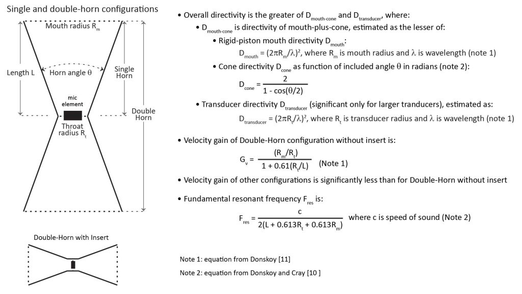
Donskoy [11] showed that the Double-Horn (DH) configuration provides significantly greater gain than the Single-Horn (SH) configuration, and due to symmetry, it seems that a DH might avoid some types of distortion that could occur with an SH (although I have no proof of that). The apparent downside, of course, is that the DH is twice as long as an SH…but depending on the length of the horn, that might not be a significant disadvantage (more on that later).

For these reasons, the rest of this AVH discussion will focus on just the DH configuration.

Double-horn with insert

The third configuration in Figure 25 (shown at the bottom left) is what Donskoy [11] refers to as a “double-horn with insert”, and he shows that it provides substantially less gain than the plain DH (without insert). Donskoy doesn’t indicate what prompted him to include this configuration in his analysis, but it seems that the insert offers additional design flexibility in the configuration of the pressure-gradient microphone. I’ll address this configuration further in an upcoming post on building AVH microphones, but won’t consider it further in this post.

Horn profiles for AVH microphones

As with an APH, a variety of horn profiles (conical, exponential, hyperbolic, etc.) can be used with an AVH. However, the literature so far addresses only conical and exponential profiles.

Donskoy [11] has shown that a conical AVH provides greater velocity gain than an equivalently-sized exponential AVH.

And the advantage of an exponential profile in an APH (a lower throat cutoff frequency for a given horn size) doesn’t apply to an AVH, because both conical and exponential AVHs have a flat low-frequency response that extends down to virtually DC.

Therefore, I conclude that there is currently no reason to consider anything but the conical profile for AVH applications

AVH microphone performance

As with an APH, there are three key performance metrics for an AVH: gain, frequency response, and directivity.

AVH velocity gain

Horn gain is more important in an AVH than an APH, for three reasons:

• One of the most compelling reasons for using an AVH is its superior low-frequency response relative to APHs and parabolic dishes. However, at low frequencies, a reasonably-sized horn provides no directivity enhancement, which means that gain is the sole benefit of an AVH microphone over a bare pressure-gradient microphone (at least at low frequencies).
• The pressure-gradient microphones used in an AVH are generally less sensitive than the pressure microphones used in an APH.
• In an APH, the pressure gain is equal to the ratio of mouth to throat areas. On the other hand, according to Donskoy [11], the velocity gain in an AVH can never exceed the ratio of mouth to throat radii…so the velocity gain of an AVH is much smaller than the pressure gain of an APH of similar size.

Thus, unlike an APH, it’s hard to have too much gain in an AVH.

Donskoy [11] shows that the gain of the conical double-horn AVH can come very close to the mouth-to-throat radius ratio, and can be estimated with reasonable accuracy using the equation shown in Figure 25.

AVH low-frequency response

All of the relevant papers show that an AVH—regardless of its horn profile—provides a reasonably flat velocity gain (and, hence, a reasonably flat frequency response) up to the horn’s fundamental resonant frequency.

Therefore, if we choose to limit the bandwidth of an AVH to below its first resonant frequency, then we don’t need any equations to predict its frequency response; all we need is Donskoy’s relatively simple equation to determine the fundamental resonant frequency (reproduced in Figure 25). The horn will have a virtually flat response below that frequency, and we can ignore the horn’s output above it.

AVH high-frequency response

As I’ve mentioned, only the paper by Buiat et al [12] discusses AVH response above the fundamental resonant frequency. The single horn they tested exhibits a broad peak in velocity gain at the predicted resonant frequency, but (at least to my eyes) the data doesn’t suggest any gain dependence on frequency due to effects other than resonance.

Extrapolating from this one data point is risky, but to me it suggests that there is no need to try to predict the wideband response of an AVH: it can be assumed to be reasonably flat except for resonance effects whose amplitudes are notoriously difficult to predict analytically.

So, if wideband operation is intended, it seems that the best that can be done is to be aware that there will be a significant response peak at the fundamental resonance, and to plan on testing to determine the shape of the peak so that it can be electronically equalized.

AVH directivity

The AVH differs from the APH in that it provides bidirectional, rather than unidirectional, directivity. But as with any sound-collecting device, that directivity will be frequency-dependent. There are two directivity regimes we need to consider, depending on the frequency range over which we intend to operate the horn.

AVH directivity below first fundamental horn resonance

If we choose to use an AVH only below its fundamental resonant frequency, then we don’t have to worry about estimating its directivity at all. That’s because a horn’s fundamental resonant frequency decreases with increasing size. For practical horn geometries, this means that the horn’s mouth will be too small at the fundamental resonant frequency to provide any directivity enhancement over the microphone element itself.

Therefore, there’s no need to attempt to quantify the directivity of an AVH operated below its fundamental resonance, because it will be essentially the same as that of the pressure-gradient microphone’s native dipole directivity.

AVH directivity at higher frequencies

As I suggested above, there’s reason to believe that the usable bandwidth of an AVH could exceed the fundamental resonant frequency. However, none of the references I found addressed directivity in the high-frequency regime.

My assumption is that a conical double-horn AVH provides high-frequency directivity in the same way as a conical APH, so that the same equations should apply (except that the AVH’s directivity will be bidirectional rather than unidirectional). Therefore, the directivity equations I’ve included in Figure 25 are the same as those I use to estimate the directivity of a conical APH.

However, the way an arriving wavefront interacts with the horn’s mouth is obviously different between an AVH and an APH, because the AVH shows no sign of the mouth cutoff frequency evident in an APH. It’s quite possible that the same phenomenon that causes this difference also affects the mouth directivity.

But how about a single-horn AVH? My intuition says it should work the same way as a double-horn from a directivity perspective, but I’m less sure because of the asymmetry.

Since I can’t find any references that address these issues, I’m going to have to build and test some AVHs myself, and will report my findings on this site when I do.

Key AVH microphone design trades

While the physics inside an AVH are seemingly more complex than for an APH, the design process for an AVH microphone is actually simpler, especially if we intend to operate it only below its fundamental resonant frequency:

• We don’t need to worry about optimizing the horn profile or size/shape for the desired low-frequency response (as with an APH), because low-frequency response isn’t an issue for AVHs.
• If we only intend to operate the AVH below its fundamental resonance, then the design process doesn’t have to address directivity, since the directivity will be the same dipole directivity as that of the pressure-gradient microphone element.

AVH microphones intended for low-frequency operation

If we intend to operate the AVH only below its fundamental resonant frequency, then the only design trade we need to consider is bandwidth versus gain: the larger the horn, the greater the gain…but the lower the resonant frequency (and hence the usable bandwidth).

We can show this trade graphically if we make a couple of assumptions:

• We need to assume a throat radius. Since horn gain is approximately equal to the ratio of the mouth radius to the throat radius, and we want both to be as small as possible to maximize the fundamental resonant frequency, we definitely want to minimize the throat radius. The minimum throat radius will be determined by the microphone radius:
  • The smallest pressure-gradient microphone capsule that’s readily available has a radius of about 3mm. However, the throat of an AVH must be left open, so we’ll assume a throat diameter of 4 mm.
• We need to assume a horn angle, which we can characterize using the ratio of mouth radius R_m to horn length L (where L is the length of each of the two horns if we’re using a Double-Horn configuration). We’ll use three values of R_m/L for this example: 1, 2, and 4.

With these assumptions, we can use the equations of Figure 25 to plot the velocity gain versus fundamental resonant frequency for each of the three horn angles:

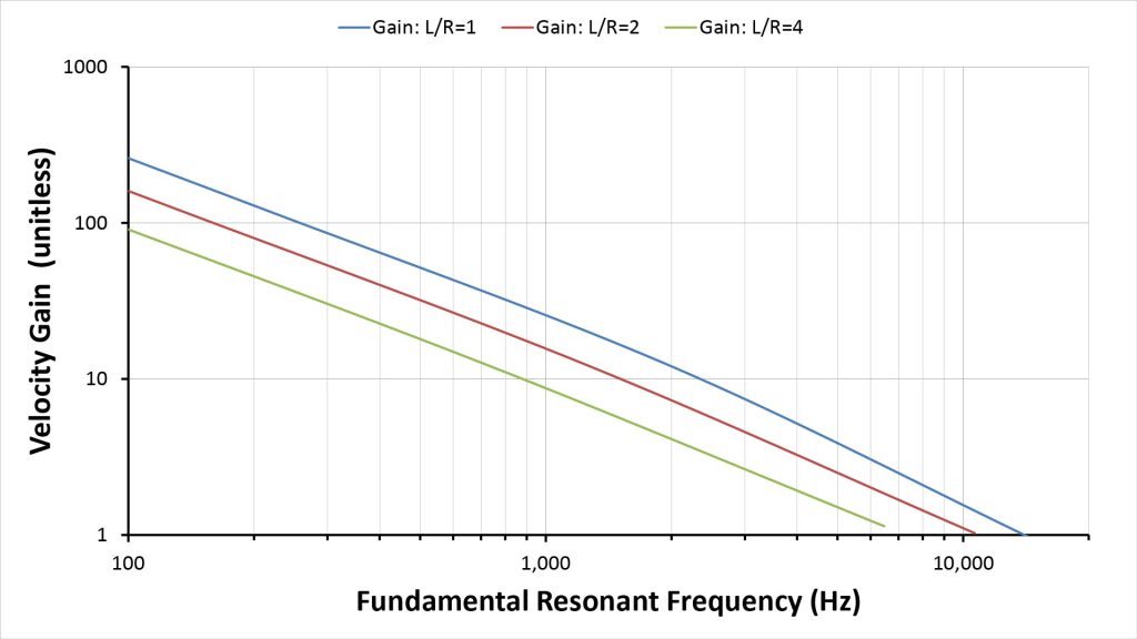
What’s immediately obvious from these curves is that, if we want to operate below the fundamental resonant frequency, an AVH provides high gain only at low frequencies.

For example, consider an AVH with an L/R_m ratio of 1 (which has the highest fundamental resonance of the three horn angles for a given gain). From Figure 26, we can conclude that:

• If we want a resonance of 10 kHz, we get a velocity gain of only 1.7 (or 2.4 dB).
• If we want a gain of 10 dB, the fundamental resonance drops to just 2.4 kHz.
• If we want a gain of 20 dB (100), the fundamental resonance is just 260 Hz.

So we’re stuck with low gain if we want to use an AVH to capture most of the voice spectrum. On the other hand, an AVH that can capture most of the voice spectrum (up to, say, 6 kHz) does have the advantage of being quite small. We can use the same equations to plot the mouth radius (which will also be the horn length) for the L/R=1 horn, like this:

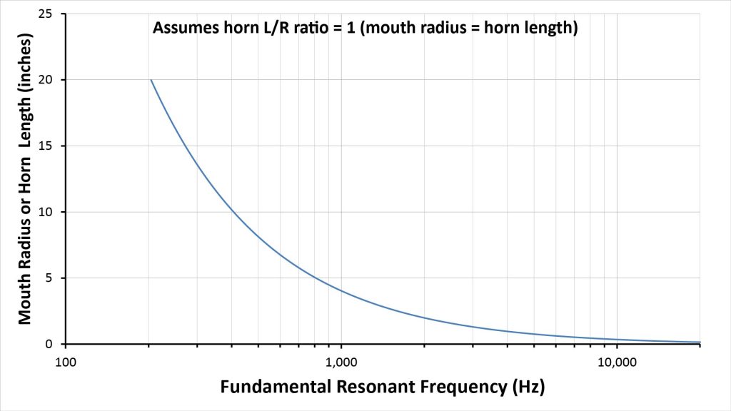
A horn with a fundamental resonance of 10 khz will have a mouth radius and length of just 0.35 inches, while a resonance of 6 kHz implies a radius and length of just 0.6 inches. The gains aren’t high (just 2.4 dB and 5 dB, respectively), but the horns are so small that these gains are effectively “free”.

AVH microphones intended for wideband operation

If an AVH can, in fact, be successfully operated at frequencies above its fundamental resonance, then the key design trade is between gain/directivity and horn size. As noted above, I’m assuming for now that a conical AVH provides the same directivity (except two-sided) as a conical APH of the same size.

The greater the desired gain and directivity, the larger the horn, and the associated equations as shown in Figure 25 are quite simple. Whether gain or directivity drives the required horn size will depend on the intended application.

Horn microphone applications

Hopefully the preceding material has given you a good idea of horn microphone theory and capabilities. But if horn microphones are useful, why are they so rare…and what are their practical applications?

Let’s take the last question first: horn microphones are potentially useful whenever acoustic gain or directivity greater than that of a conventional studio microphone is needed. That makes them potential alternatives to shotgun and parabolic microphones. By the way, I have a section devoted to comparing horn, parabolic, shotgun, and array microphones in my post on long-range directional microphones.

APH microphone applications

When they were first developed, horn microphones were most useful in short-range applications (such as in old-fashioned telephone mouthpieces), where an APH’s pressure gain could compensate for the poor sensitivity of early microphones.

Today, microphone sensitivity is not an issue, so the APH’s main benefit is directivity, not gain (although the gain is still useful). In this sense, the APH falls neatly between parabolic and shotgun microphones:

• An APH microphone provides less directivity and gain than that of a parabolic microphone of the same volume—but is more physically robust, easier to build, and potentially much cheaper.
• A DIY APH microphone is bulkier than a shotgun microphone of the same length, but is far cheaper and provides substantial gain (while the shotgun provides no gain) along with greater greater directivity.

We can get a better idea of the potential applications of APH microphones by comparing them to typical parabolic and shotgun microphones from a maximum-range perspective. Exemplar microphones for such a comparison are listed in the following table.

Type	Description	Notes
Parabolic	26-inch dish with dish efficiency of 0.6	Typical of commercially-available parabolic microphones; largest parabolic mic that isn’t prohibitively difficult to handle
Shotgun	20-inch interference tube with hypercardioid element	Typical of modern extra-long shotgun mics (such as the Sennheiser MKH-8070) which use a hybrid hypercardioid/interference-tube arrangement
Horn	13-inch conical Acoustic Pressure Horn (APH)	Small DIY horn microphone using an off-the-shelf cheerleader’s megaphone
Horn	25-inch conical Acoustic Pressure Horn (APH)	Medium DIY horn microphone using an off-the-shelf cheerleader’s megaphone
Horn	32-inch conical Acoustic Pressure Horn (APH)	Large DIY horn microphone using an off-the-shelf cheerleader’s megaphone
Horn	12-inch exponential Acoustic Pressure Horn (APH) with flare constant of 0.35	Small DIY horn microphone using an inexpensive off-the-shelf speaker horn (with a retail cost of less than $20)
Horn	12-inch exponential Acoustic Pressure Horn (APH) with flare constant of 0.6	Slightly larger DIY horn microphone using an inexpensive off-the-shelf speaker horn (with a retail cost of less than $20)

Estimating the maximum range

Accurately estimating the maximum pick-up range of a microphone involves estimating the Signal-to-Interference-plus-Noise Ratio (SINR) at the microphone output as a function of frequency, and then determining the range at which that SINR-versus-frequency profile just barely provides the required signal quality. This is not a trivial process, which is why I’ve written a series of posts on it:

• Predicting microphone performance—Part 1: what is microphone SINR?
• Predicting microphone performance—Part 2: using the SINR
• Predicting microphone performance—Part 3: microphone range prediction

The first two posts introduce the SINR, while the third describes several SINR-based methods for microphone range prediction. The range estimates given below were obtained using the most sophisticated of these methods, which is based on SINRs evaluated in eleven frequency sub-bands across the audio spectrum. This enables it to comprehend not just the frequency-dependence of directivity and gain, but also differing spectral characteristics of the target sound and ambient noise. The range estimates below are for what I call the “General” microphone usage scenario, which includes the following assumptions about the target sound and ambient noise:

• The assumed target sound is human voice at a normal conversational volume of 70 dBA at 1 foot (see Predicting microphone performance—Part 1: what is microphone SINR? for the assumed spectral characteristics). This is the same target sound model assumed in three of the other application scenarios of Table 1, including the Surveillance scenario.
• The assumed ambient noise is what I call the Indoor Medium noise profile with a broadband SPL of 35 dBA (see Predicting microphone performance—Part 1: what is microphone SINR? for the assumed spectral characteristics). The Indoor Medium noise profile is very similar to the Outdoor Rural profile assumed in my Surveillance scenario.

Range prediction also requires some assumptions about the required signal quality (as determined by the SINR-versus-frequency profile) at the output of the microphone. The range estimates given below assume two different levels of required signal quality:

• “75-percent intelligibility” represents the minimum signal quality needed when capturing voice for surveillance or sports applications.
• “Medium fidelity” represents the minimum signal quality needed for general-purpose voice capture (such as for videography, business communications, or social media applications).

The following bar charts show the estimated range for the microphones of Table 2 in the General scenario, for both the “75-percent intelligibility” and “medium fidelity” signal-quality thresholds:

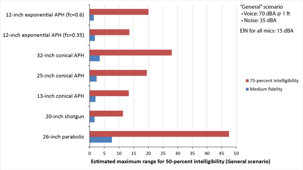
As the figure shows, none of the exemplar APH microphones can match a 26-inch parabolic microphone for sheer range.

However, the 32-inch conical APH provides enough range to be a viable alternative to a parabolic microphone for some applications. And a 32-inch cheerleader’s megaphone can be purchased for less than $50 (and can be built from scratch even more cheaply), and is much more robust than a parabolic reflector.

Also note that all of the APH microphones comfortably out-perform the 20-inch shotgun microphone (which is typical of today’s “long-range” shotgun microphones) for capturing barely-intelligible voice (per the “75-percent intelligibility” bars).

If a higher-quality signal is needed, then all but one of the APH microphones still out-perform the shotgun microphone (per the “medium fidelty” bars). The lone exception is the 12-inch exponential APH with a flare constant of 0.6. The high flare constant of this horn results in a relatively high cutoff frequency, which significantly limits its maximum range against voice and music.

However, if used to capture bird songs or bat vocalizations, this particular horn would have a much longer range than all but the 26-inch parabolic microphone due to its relatively large mouth area—and at only a fraction of the cost and size of a true 26-inch parabolic reflector.

So, the APH microphone can be much more cost-effective than parabolic or shotgun microphones in two specific applications:

• As a parabolic microhone alternative when cost and robustness are more important than maximum pick-up range.
• As a shotgun-microphone alternative when cost and pick-up range are more important than compactness.

AVH microphone applications

Unlike an APH, an AVH offers a low-frequency response down to near zero frequency, but has bidirectional (rather than unidirectional) directivity with much less gain than an APH.

The fact that an AVH has a bidirectional polar pattern might seem to be a serious disadvantage for long-range pickup. However, if the ambient noise is isotropic, the bidirectional polar pattern will increase the noise level by only a modest 3 dB relative to a unidirectional pattern. Further, a bidirectional pattern is advantageous for some applications.

So where would an AVH be useful? Here are some ideas:

• Low-noise bidirectional studio microphone. The velocity gain of an AVH reduces the effective self-noise of its microphone capsule one-for-one. So, for example, a 10 dB velocity gain would make a pressure-gradient microphone capsule with an SNR of 70 dB sound like one with an SNR of 80 dB.
• Infrasound sensing and capture. An AVH’s high gain at low frequencies can facilitate sensing and recording of low-level infrasound signals. This is admittedly a pretty esoteric application, but if you happen to need to sense infrasound, an AVH could be your best option.
• Infrasound source localization. While an AVH (like any directional microphone) provides negligible directivity at low frequencies, a bidirectional (figure-8) pattern has off-axis nulls that are theoretically infinitely deep. So, if you want to determine the direction of arrival of an infrasound signal, you can rotate an AVH to find the minimum signal level; the bearing to the source will then be 90 degrees off the AVH axis. You don’t need an AVH to do this if the signal is strong, but the AVH gain can be very useful if the signal level is weak.

I have several posts on DIY APH and AVH microphones in the pipeline, so stay tuned!

Why are horn microphones so rare?

So why aren’t horn microphones more popular? Early in this post I mentioned a few potential reasons for their relative rarity, including the fact that the original motivation for horn microphones (the limited sensitivity of then-available microphone elements) ceased being an issue decades ago. Another likely reason is that other directional microphones (shotgun microphones, and to a lesser extent parabolic microphones) are already well-entrenched.

But the only reason that would really matter would be the existence of some kind of serious performance issue. As I’ve discussed, resonance is definitely a potential issue with AVH microphones. But resonance is thought by some audiophiles to be audible in horn speakers (which use acoustic pressure horns), so it could also be an issue APH microphones.

But even if resonance is an issue, there might be ways to mitigate it…through both horn design and electronic equalization.

The only way to know for sure is build some horn microphones and test them out…which is exactly what I’m going to do!

References

1. J. Dinsdale, “Horn Loudspeaker Design,” originally printed in Wireless World, March 1974. Available at http://www.p10hifi.net/planet10/TLS/downloads/Dinsdale-Horns-3parts.pdf [accessed January 2022].
2. Arthur Gordon Webster, “Acoustical Impedance and the Theory of Horns and of the Phonograph,” in Proceedings of the National Academy of Sciences, July 1, 1919 5 (7) 275-282. Available at https://www.pnas.org/content/pnas/5/7/275.full.pdf [accessed January 2022].
3. Edward Eisner, “Complete Solutions of the “Webster” Horn Equation,” in The Journal of the Acoustical Society of America 41, 1126 (1967). Available at https://asa.scitation.org/doi/10.1121/1.1910444; cost is $33 for non-members of JAES [accessed January 2021].
4. Richard C. Morgans, “Optimisation techniques for horn loaded loudspeakers,” Ph.D thesis, The University of Adelaide, South Australia, 2005. Available at https://hdl.handle.net/2440/41350 [accessed January 2022].
5. Harry F. Olson, Elements of Acoustical Engineering. New York: D. Van Nostrand and Company, 1947. Available at https://archive.org/details/in.ernet.dli.2015.239408/page/n1/mode/2up [accessed January 2022].
6. Daniel J. Mennitt, Kurt M. Fristrup, Branislav M. Notaros, “Characterization of gain and directivity of exponential horn receivers,” in J. Acoust. Soc. Am. 142 (5), November 2017. Available at https://www.engr.colostate.edu/~notaros/Papers/JASA_Acoustic_Horns.pdf [accessed January 2022].
7. P.M. Morse, and K.U. Ingard. Theoretical acoustics. McGraw-Hill Book Company, New York, 1968.
8. Ronald M. Aarts and Augustus J.E.M. Janssen, “Comparing sound radiation from a loudspeaker with that from a flexible spherical cap on a rigid sphere ,” in JAES Volume 59 Issue 4 pp. 201-212; April 2011. Available at https://www.aes.org/e-lib/browse.cfm?elib=15925 (cost is $33 for AES non-members). Similar paper is freely available at https://www.univie.ac.at/nuhag-php/janssen/data/p182b.pdf [accessed January 2022].
9. Dimitri M. Donskoy and Benjamin A. Cray, “Acoustic particle velocity horns,” in J. Acoust. Soc. Am. 131 (5), May 2012. Available at https://asa.scitation.org/doi/full/10.1121/1.3702432; cost is $33 for non-members of JAES [accessed May 2021].
10. Dimitri M. Donskoy and Benjamin A. Cray, “Horns as particle velocity amplifiers,” in J. Acoust. Soc. Am. 130 (5), November 2011. Available at https://asa.scitation.org/doi/10.1121/1.3642644; cost is $33 for non-members of JAES [accessed January 2021].
11. Dimitri M. Donskoy, “Directionality and gain of small acoustic velocity horns,” in J. Acoust. Soc. Am. 142 (6), December 2017. Available at https://asa.scitation.org/doi/10.1121/1.5016817; cost is $33 for non-members of JAES [accessed June 2021].
12. Martina Buiat, Davide Bonsi, Paolo Bruschi, Fosca Fimiani, Massimo Piotto, Domenico Stanzial, “Application of acoustic horns for the amplification of a p-v probe velocimetric signal,” presented at Forum Acusticum, Krakow, Poland, September 2014. Available at https://www.fe.infn.it/acustica/pubblicazioni/Conferenze/Forum%20Acusticum%202014/R05A_2.pdf [accessed January 2022].
13. Bjorn Kolbrek, “Horn Theory: An Introduction, Part 2,” AudioXpress, March 2008. Available at https://kolbrek.hornspeakersystems.info/index.php/publications [accessed January 2022].