Predicting microphone performance—Part 1: what is microphone SINR?

What is microphone SINR and how do you calculate it? Designing—and properly using—a microphone often calls for a way to predict microphone performance. This post introduces the most useful metric for that purpose: the Signal-to-Interference-plus-Noise Ratio (SINR).

Microphone performance and why we’d want to predict it

The purpose of a microphone is to convert sound from a particular source to an electrical signal, which can then be transmitted or recorded for a particular application.

Thus, we can define microphone performance as the degree to which the quality of the output signal suits the needs of the application.

Per this definition, microphone performance depends on the characteristics of the sound, the characteristics of the microphone, and the way the microphone is used. Some of these factors will be under our control, and some won’t.

So, one motivation for microphone performance prediction is to ensure that we can manipulate the factors under our control so that the quality of the signal is sufficient for the intended application.

Examples of questions that can be answered by a microphone performance prediction (and only a microphone performance prediction) are the following:

• How well will a particular microphone work in the intended application?
• Which of two microphone designs will perform better in a given application?
• How far away can a particular microphone be placed from the source while still providing adequate signal quality for the intended application?

I’ll address how to answer such questions in other posts in this series. In this part one, I’ll focus on the key metric for microphone performance prediction: the Signal-to-Interference-plus-Noise Ratio (SINR).

A key assumption: we’re going to use the microphone properly

Any microphone performance prediction has to make assumptions about how the microphone will be used, and it makes sense to assume that all the factors that can be controlled will be controlled to maximize performance. There are two things in particular that we can and should do when using a microphone:

• We can avoid significant Total Harmonic Distortion (THD) in the signal by ensuring that the Sound Pressure Level (SPL) at the microphone’s diaphragm is no greater than the microphone’s distortion-free SPL spec. This is easy to do unless the microphone is located excessively close to a loud source (or a microphone with an inappropriately low SPL rating is being used).
• We can frequency-equalize the microphone’s output to ensure that its spectrum has the desired shape. Even though this desired spectrum might not be the same as the spectrum of the sound we’re trying to capture, a reasonable assumption for performance prediction is that the spectra should match; in other words, we can assume that we want the equalized frequency response to be flat. As explained in my post on the 4 key microphone specifications, this is easy to do and removes microphone frequency response as a potential performance issue.

If we do these things (and we certainly should), then the only thing that will significantly limit microphone performance is noise—either actual acoustic noise from the environment (aka ambient noise) or electrical noise generated in the microphone itself (Effective Input Noise, or EIN). And that observation sets the stage for our SINR discussion.

The key microphone performance metric: the Signal-to-Interference-plus-Noise Ratio (SINR)

Assuming that we employ good microphone practice to avoid THD and frequency-response issues, we can quantify the quality of the microphone output with a single metric: the Signal-to-Interference-plus-Noise Ratio (SINR).

The concept of microphone SINR is simple: it’s just the ratio of the power of the desired component of the output signal to the power of the undesired component of the output signal:

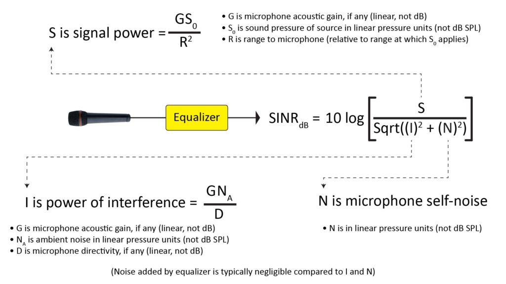
Note that the equalization (whether positive or negative) affects the numerator and denominator of the SINR equally, and therefore has no effect on the ratio.

The desired component (the numerator of the SINR) is due to the sound we’re trying to capture. Its power depends on the Sound-Pressure Level (SPL) of the sound at its source, the distance from the source to the microphone, and any acoustic gain provided by the microphone (such as from a parabolic reflector).

The power of the undesired component (the denominator of the SINR) depends on the root-sum-square of the ambient acoustic noise (after any acoustic gain or ambient noise suppression provided by the microphone) and the microphone self-noise. The root-sum-square, and not the arithmetic sum, determines the power of the undesired component because noise powers add incoherently, not coherently.

The microphone SINR thus takes into account all of the variables that can affect sound quality (assuming, again, that THD is not an issue and that potential frequency-response issues have been mitigated through appropriate equalization).

The quantity expressed by the microphone SINR could also be thought of as just plain “SNR”, where N refers to the root-sum-square of the ambient noise and microphone self-noise. However, “SNR” is also a term often used in microphone specifications, wherein the “N” refers just to microphone self-noise. So, the term “SINR” is not only more descriptive, it also avoids confusion with the conventional SNR spec.

In my post on the 4 key microphone specifications, I discuss how we can eliminate microphone EIN as a potential performance issue by ensuring that it’s comfortably below the interference level. If we’re able to do this—and we often are—then the EIN can be neglected and the SINR reduces to just the Signal-to-Interference Ratio (SIR). That’s very convenient, because it eliminates the need for the root-sum-square in the denominator and allows all the variables to remain in dB-SPL or dBm units. However, there are situations in which the EIN does significantly affect the SINR, so I’m going to deal with the complete SINR in this post.

The microphone SINR variables are referenced to the input of the microphone

While the SINR applies to the electrical output signal of the microphone, the sound-pressure variables that determine it can be referenced to either the output of the microphone (in which case they might be in units of volts squared), or to the input of the microphone (in which case they might be in units of SPL or Pascals).

A good example of an output signal characteristic that’s referred to the input of a microphone is EIN. The EIN refers to the electrical self-noise in the output of a microphone, but is expressed as the level of a fictitious acoustic noise (in dB SPL) at the mic’s diaphragm. That’s convenient because it puts the EIN in perspective, enabling quick comparison with an actual ambient noise level.

The resulting SINR is the same whether the sound-pressure variables are input-referenced or output-referenced, but the variables have different meanings as shown in the following table:

Variable	Meaning when referenced to the microphone output	Meaning when referenced to the microphone input (the incident sound)
Signal	Component of the electrical output signal attributable to the desired sound; depends on microphone sensitivity as well as signal SPL	Pressure of the desired sound at the microphone; expressed in either dB-SPL or linear pressure units (Pascals)
Interference (ambient noise)	Component of the electrical output signal attributable to ambient noise; depends on microphone sensitivity as well as interference SPL	Pressure of the ambient noise at the microphone diaphragm after acoustic noise suppression (if any); expressed in either dB-SPL or linear pressure units (Pascals)
Noise	Component of the electrical output signal attributable to the microphone self-noise	Equivalent Input Noise (EIN), which is defined as the SPL of a fictitious acoustic noise at the microphone diaphragm that would yield the same output level as the microphone’s electrical self-noise; expressed in either dB-SPL or linear pressure units (Pascals)

It’s more convenient to reference these quantities to the microphone input (which is what’s usually done), and that’s what Figure 1 assumes.

Notice that when we do this, the microphone sensitivity—perhaps surprisingly—does not factor into the SINR. It does affect the microphone output level (the lower the sensitivity, the lower the output level for a given SPL). But if the downstream device has a reasonably quiet front-end with the appropriate amount of gain, then microphone sensitivity has only a minor (and usually negligible) impact on sound quality.

The sound-pressure variables of Figure 1 are in linear pressure units, not dB-SPL

Per Table 1, we can express the sound-pressure variables as either dB-SPL or in linear pressure units (Pascals). Sound pressures are typically expressed in dB-SPL, but the incoherent addition of noise powers in the SINR denominator of Figure 1 requires that the noise powers be expressed in linear pressure units. I could have shown the conversion between dB-SPL and Pascals in Figure 1, but that would have made the figure much busier, so the variables are in Pascals.

We can convert between dB-SPL and Pascals as follows:

• dB_SPL = 20log(p/20 μPa), where p is the absolute pressure
• p = (20 μPa) ∗ 10^(dB_SPL/20)

The microphone SINR depends on bandwidth-integrated variables

The signal, ambient noise, and microphone EIN all depend on the bandwidth over which they’re evaluated.

We can evaluate the variables over an entire bandwidth of interest (such as the entire audible bandwidth, which extends from ~20 Hz to ~20 kHz, or the voice bandwidth, which extends from ~100 Hz to ~8 kHz), or we can evaluate them over one (or more) smaller sub-bands within the bandwidth of interest. Both approaches can be useful in microphone performance prediction.

The microphone SINR varies with frequency

All of the quantities that determine the SINR typically vary with frequency, and they generally won’t all vary in the same way. This means that the SINR itself will generally vary with the center frequency of whatever bandwidth is used for the evaluation.

Thus, an SINR calculated over an entire bandwidth of interest (say the entire audio bandwidth) could significantly understate or overstate the SINR at any given frequency within that bandwidth. That’s one reason why we might want to evaluate the SINR over one or more sub-bands within the bandwidth of interest.

Choosing the sub-band center frequencies and bandwidths for SINR estimation

If we’re going to evaluate the SINR variables over a sub-band within the overall bandwidth of interest, how many sub-bands should we use, what should be their center frequencies, and how wide should the sub-bands be? In general, there will be one of three answers to those questions, depending on the microphone we’re trying to model and the object of our SINR estimation:

• If we’re modeling a microphone that has a flat frequency response and a flat directivity-versus-frequency characteristic, and if we’re trying to capture sound that’s expected to have a flat spectrum (such as live music), then a single SINR value evaluated over the entire bandwidth of interest will generally suffice.
• Otherwise, we have three choices:
  • If we know the frequency at which the SINR is going to be the poorest (it’s usually the lowest frequency in the bandwidth of interest), then a single SINR value for a sub-band centered at that frequency will provide a conservative estimate of the signal quality. However, such an estimate will typically be too conservative to be of much use.
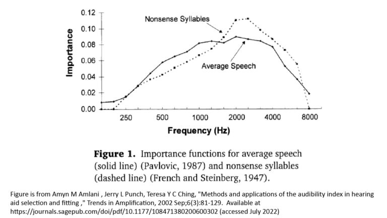
  • If there is a single sub-band that contributes the most to the quality of the sound we’re trying to capture, then a single SINR value over that sub-band can be useful quality metric. In fact, the SINR over an octave-wide sub-band centered at 2 kHz can be a very useful metric for assessing the quality of voice captured by a microphone.
  • If we want an even better measure of signal quality, we can evaluate the SINR over multiple sub-bands over the bandwidth of interest. Audio spectra are often measured with sub-bands that are only one-third octave wide (or even narrower), but the spectral granularity afforded by such narrow sub-bands is overkill for SINR estimation purposes; full-octave sub-bands will suffice for most purposes. However, using multiple sub-bands raises an obvious question: how do we weigh the corresponding SINR values to obtain an overall measure of quality? That’s beyond the scope of this post, but I discuss it in part 2 of this series.

But regardless of how many sub-bands we use or their center frequencies, the process of estimating each SINR value is the same.

The sound pressures can be unweighted or A-weighted, depending on how the SINR is used

When using the SINR to predict microphone performance, we must account for the ear’s distinctly non-flat frequency response in either of two ways:

• If we’re characterizing the quality of the microphone’s output signal with just a single SINR value evaluated over a wide bandwidth, then all of the sound-pressures used in the SINR equation must be A-weighted.
• If we’re using one (or more) SINR values evaluated over a narrow sub-band, then all of the sound-pressures can be either A-weighted (in dBA) or unweighted (in dBZ), depending on how the SINR is to be interpreted. The multiple-SINR approach I use (and describe in detail in Part 2 of this series) uses unweighted sound-pressures, as does the rest of this post.

A deeper look at the microphone SINR variables

With that general overview of the SINR out of the way, we’re now ready to take a deeper look at each of the variables that go into the SINR.

The SINR numerator: the desired component of the output signal

Referring again to Figure 1, the signal power S (the component of the microphone output attributable to the desired sound) is found as:

• S = S₀G/R², where
  • S₀ is the mean pressure of the desired sound at known distance R₀ (such as 1 foot or 1 meter) from its source;
  • G is the gain, if any, provided by the microphone;
  • R is the ratio of the distance between the source and the microphone to R₀ (for example, if the distance between the source and the microphone were 10 feet and R₀ were one foot, R would be 10).

The mean pressure level of the desired sound

The pressure of the sound we want to capture with a microphone usually varies in time, ranging from some minimum to some maximum; the difference between the minimum and maximum pressures is the sound’s dynamic range. However, from the SINR perspective, the minimum and maximum pressures aren’t very meaningful; instead, what we care about is the mean (average) sound pressure.

The pressure of the sound we want to capture can also vary significantly with frequency; in other words, it can have a non-flat spectrum, and that spectrum can also vary in time. For SINR purposes we generally care about the Long-Term Average Spectrum (LTAS) of the sound, which is the spectrum over a time-window that can range for tens of milliseconds to tens of seconds.

Music

If we’re capturing live music with our microphone, then the mean pressure and LTAS will depend on the type of music and are hard to predict. For live music, it’s usually best to assume a flat LTAS for SINR estimation purposes.

If we’re recording non-live music (played over a speaker), then the LTAS will be affected by the sound-system’s frequency response (and, particularly, the frequency response of the speaker). However, this is a relatively rare scenario, and I won’t consider it further in this post.

Voice

Unlike the case with live music, the mean pressure and LTAS of voice can be predicted with enough accuracy for useful SINR calculations.

As an example of voice spectra, the following figure, from Lienard [1], shows the LTAS of voice from two speakers (one male, one female) as a function of Vocal Strength (VS) ranging from casual speech to a shout:

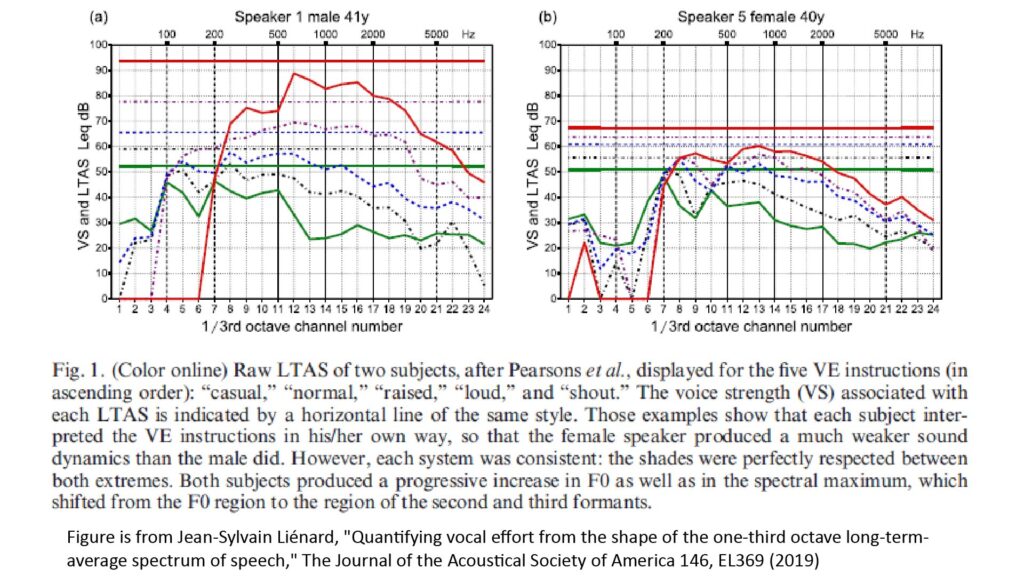
Note that, like most sound-pressure data, the sound pressures of Figure 2 are in SPL (in dBZ), so we’ll have to convert them to Pascals before using them in the SINR equations of Figure 1

Each SPL value for the solid-line curves of Figure 2 represents the SPL over a one-third-octave sub-band, while the dotted lines represent the SPLs over the whole voice bandwidth. As we would expect, the SPLs increase as the voice gets louder, but the shapes of the one-third-octave LTAS curves also change; the SPLs get shifted to higher frequencies.

Based on this and similar data, I’ve developed three voice models that I use for microphone range prediction: one for casual speech, one for a loud speaking voice, and one for a shout. The models are depicted in the following figure:

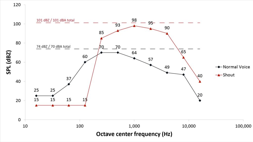
Note that the SPLs of Figure 3 are much greater than those of Figure 2. There are two reasons for this:

• Figure 3 is based on full-octave sub-bands instead of 1/3-octave sub-bands, because I think the wider sub-bands are more practical choice for SINR estimation purposes. The SPLs are therefore greater by 10*log(3) or 4.77 dB due to the 3X wider sub-band bandwidth.
• I usually use SI (metric) units for most purposes, but for some reason I used feet in the earliest posts on this blog…so, for consistency, I’m sticking with feet as the primary unit of distance. Accordingly, the SPLs of Figure 3 assume an R₀ (distance from speaker) of 1 foot, while Figure 2 was based on a 1 meter R₀; the shorter range further increases the SPLs by an additional 10.3 dB.

The microphone gain, if any

The previous two variables (the source pressure S₀ and the relative range R) are independent of microphone design. But the third variable—the gain G (if any)—is a microphone attribute.

Note that the gain we are talking about here is not the kind of gain provided by an amplifier or attenuator downstream of the microphone element. Such downstream gain affects both the signal level and the microphone EIN. Instead, the gain we’re referring to here affects only the signal level without affecting the microphone EIN. There are several mechanisms that can provide such gain:

• Negative gain (attenuation) can be provided by a foam block or similar material placed in front of the diaphragm; this can be useful to increase the SPL-handling capacity of a sensitive microphone.
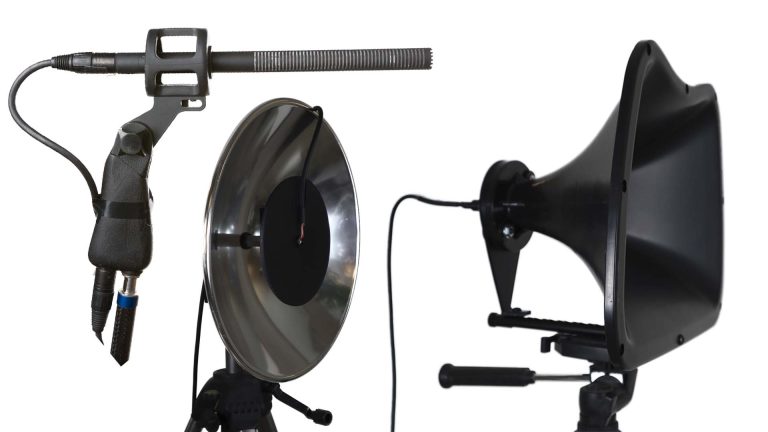
• Positive gain can be provided by a reflector or a horn; probably the most familiar example of a gain-producing device is a parabolic reflector.
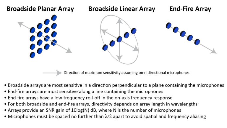
• Positive gain can also be provided by summing the outputs of multiple microphone elements in an array configuration. This causes the signals to add coherently while the noise adds only incoherently. By the way, I have a post on how array microphones work if you’re interested in the subject.

Depending on the mechanism, the gain can be either flat with frequency or, more likely, frequency-dependent. For example, the curve in the following figure plots the gain versus frequency for a parabolic dish:

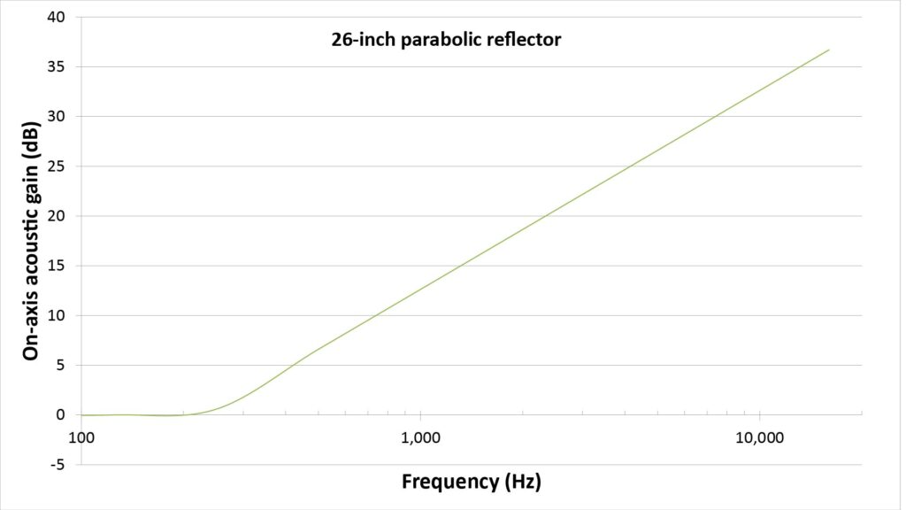
Note that Figure 4 shows the gain in dB due to its wide dynamic range (the curve wouldn’t fit on a linear scale), whereas the SINR equations of Figure 1 expect the gain as a linear factor.

By the way, if you’ve read my post on the 4 key microphone specs, you might have noticed that it didn’t cover gain. That’s because only specialized microphones (such as the parabolic and horn microphones mentioned above) provide significant gain. However, those are exactly the types of microphones for which we might want a SINR prediction, which is why I’m addressing gain in this post. A discussion of how to estimate the gain provided by those devices is beyond the scope of this discussion, but see my posts on parabolic microphones and horn microphones if you’re interested in the details.

The relative distance R between the source and microphone

The second variable that determines the net signal level in the SINR is the distance between the source and the microphone.

In general, sound spreads outward spherically as it travels, so the SPL at the microphone will be less than the SPL at the source by an amount given by the inverse-square law. There are conditions in which the inverse-square law overstates the loss with distance (specifically, when the sound is confined so that it can’t expand spherically, or when the distance is less than wavelength or so from the source), but for most applications it’s safe to assume that the inverse-square law does apply.

In the SINR equation of Figure 1, the inverse-square law appears as R² in the denominator of the signal-power equation.

The SINR denominator: the undesired component of the output signal

Now we’ll shift our attention to the denominator of the SINIR, which represents the undesirable component of the output signal. As shown in Figure 1, the denominator of the SINR has three components: the acoustic interference I and the net electrical noise N.

Acoustic interference

The denominator of the SINR is usually dominated by acoustic interference (unwanted sounds). There are three main sources of acoustic interference:

• Every indoor and outdoor environment has an ambient noise floor that represents the minimum interference level we can expect in that environment. Typical drivers of this noise floor include HVAC systems (in indoor environments) and road traffic (in both indoor and outdoor environments). The resulting ambient noise is typically reasonably homogeneous (invariant with position) and isotropic (invariant with direction), which makes it relatively easy to address for SINR prediction purposes.
• Depending on what’s happening in the environment, there are often additional noise sources that dramatically raise the interference level above the noise floor. For example, the interference level in an occupied room can be much higher (by ~10 to 20 dB) than the noise floor in an unoccupied room due to the activities of the occupants. This additional noise is usually both inhomegeneous and anisotropic and its spectrum can vary widely depending on what’s causing it, which makes it extremely difficult to predict without actual measurements.
• In an indoor environment, reverberation of the desired sound from room surfaces can be well above the noise floor. However, unlike the other potential sources of interference, the effects of reverberation aren’t necessarily negative: depending on its amplitude and decay time, reverberation can make the sound seem muddy and indistinct—but it can also add a sense of richness to the sound. Reverberation is usually inhomogeneous and anisotropic, so its effects are hard to predict without actual measurements.

Since the ambient noise floor is always present and relatively easy to characterize, any microphone SINR estimate can and should address it. On the other hand, the other sources of interference aren’t always relevant…and when they are, they’re a lot harder to predict.

Therefore, I’m going to consider only the ambient noise floor in this discussion. If you do expect significant levels of the other types of noise, the best way to obtain a reliable prediction of SINR is to actually measure the net interference level in the environment of interest. You can then use that interference level to predict the SINR for various microphone types and source-to-microphone distances.

The interference level due to ambient noise

Referring again to Figure 1, the interference level due to ambient noise is found as:

• I = GN_A/D, where
  • G is the microphone gain, if any (as previously described);
  • N_A is the mean pressure of the ambient noise; and
  • D is the directivity, if any, provided by the microphone.

Ambient noise pressure

I’ll discuss the salient ambient noise characteristics shortly. First, however, there is a method of specifying ambient noise pressure that’s worth reviewing, because you’ll probably run across it while looking for ambient noise info online.

The Equivalent Continuous Sound Pressure Level (LEQ SPL)

Like the desired sound we want to capture, ambient noise sometimes fluctuates in time. However, unlike the desired sound, simply taking the mean (average) pressure over an interval isn’t the preferred way to characterize fluctuating ambient noise. Instead, a concept known as the equivalent continuous sound pressure level is typically used.

The concept of equivalent continuous sound pressure is based on the fact that the product of time and acoustic power is energy. Equivalent continuous sound pressure levels are quoted as an LEQ SPL, in either dBA or dBZ. LEQ SPL represents the fictitious continuous SPL that would yield the same acoustic energy as the actual fluctuating SPL over a specified time interval, such as 30 seconds.

LEQ SPL turns out to be better than the mean SPL in predicting the effects of acoustic noise on the risk of long-term hearing damage. Thus, the use of LEQ is often mandatory when measuring SPLs for noise-compliance purposes. However, for most types of ambient noise of concern in microphone applications, there isn’t much difference between the simple average SPL and LEQ SPL.

In fact I consider the average and LEQ noise SPLs to be interchangeable for the purposes of predicting microphone SINR.

Indoor ambient noise

There are two types of information that can help us predict indoor ambient noise characteristics for SINR estimation purposes:

• Prescriptive information on how quiet various interior spaces should be, in the form of noise curves used by architects and acousticians. A noise curve specifies the maximum allowable SPL of background noise as a function of frequency for a room to qualify for a particular noise rating. Various noise curves have been developed over the years, but one common feature is that the allowable noise SPL decreases by about 5 dB per octave over most of the audible spectrum. A good overview of noise curves and their use is provided by Tocci [2].
• Descriptive information in the form of noise measurements of actual interior spaces. Unfortunately, there aren’t a lot of ambient noise measurements for actual interior spaces available online for free. However, one such resource is the paper by Rakerd et al [3].

Because noise curves are prescriptive, the actual noise in a room that qualifies for a particular noise rating can be much lower at certain frequencies than allowed by the corresponding curve, and the shape of the actual noise versus frequency curve typically differs significantly from that of the closest Room Criteria curve.

For example, the following curve compares several Room Criteria Mark II curves against the SPL I measured deep in the interior of an office building after work hours:

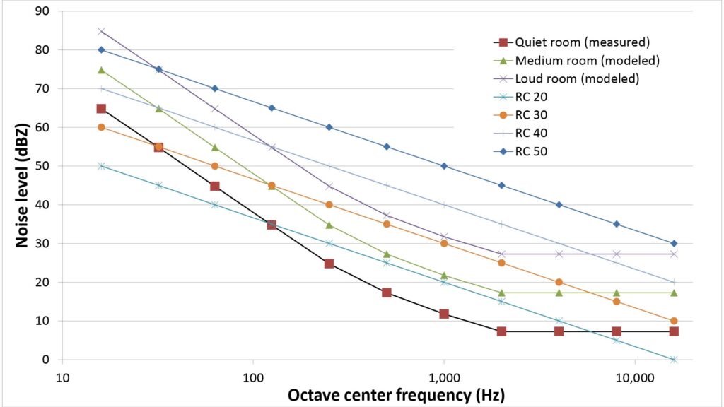
The noise I measured was up to 10 dB lower than the relevant (RC-30) noise curve in the heart of the voice spectrum (around 2 kHz). Further, this isn’t unusual in my experience; most of the unoccupied rooms in large modern office buildings I’ve measured have been relatively quiet at the middle frequencies.

Accordingly, I usually don’t use the RC Mk II curves for my own performance predictions; rather, I use three other curves shown in Figure 5:

• I use the curve labeled “Quiet room (measured)”, which I actually measured in the interior of a quiet office building after-hours, for performance projections for the quietest indoor spaces (such as recording studios).
• I use the curve labeled “Medium room (modeled)”, which is very similar to other spectra I’ve actually measured, for performance projections for indoor spaces of average loudness.
• I use the curve labeled “Loud room (modeled)”, which is very similar to other spectra I’ve actually measured, for performance projections for loud interior spaces.

Outdoor ambient noise

While most communities have noise ordinances to limit outdoor noise, there are no outdoor noise curves analogous to the room noise curves discussed above. Further, there are so many variables (such as weather and proximity to major roads) that outdoor ambient noise spectra vary over a wider range than indoor ambient noise spectra.

As a result, accurate prediction of the outdoor ambient noise spectrum in a given environment is difficult without actual measurements, and even bounding the potential spectra in various environments is a challenge.

One source of measured outdoor noise spectra is a paper by Albert and Decato [4]; the following figure shows the noise spectra reported therein for urban and rural environments, along with the spectra I use for my own performance projections:

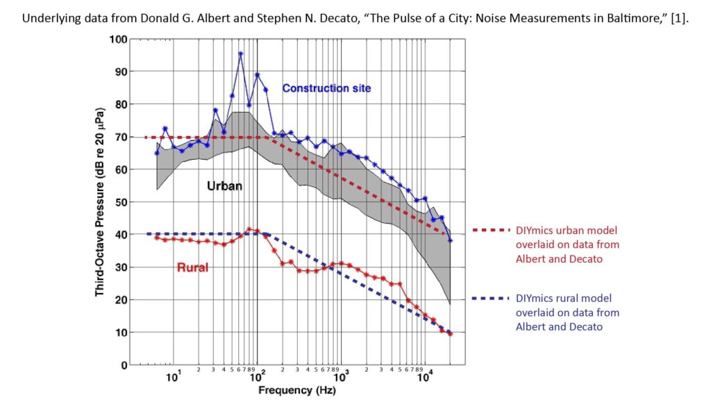
The outdoor noise spectra I use in my own SINR projections are actually 4.77 dB greater than those shown in Figure 6; I subtracted those 4.77 dB for purposes of comparison with the third-octave spectra reported by Albert and Decato.

Gain

As previously discussed, a microphone can have gain which increases or decreases the SPL of the incident sound, and by definition such gain applies to ambient noise as well as the signal. The same is true of any equalization applied to the microphone output: it applies to both the signal and interference components.

Ambient noise suppression

The final variable that determines the ambient noise component at a microphone’s output is any ambient noise suppression provided by the microphone.

There is really only one microphone attribute that can significantly reduce the impact of ambient noise: an anisotropic polar response.

Depending on the spatial distribution of the ambient noise, a microphone with an anisotropic polar response can be used to suppress the noise in either of two ways:

• If the ambient noise is isotropic, the direction of the microphone’s maximum sensitivity can be pointed toward the desired sound. The ambient noise suppression is then given by the microphone’s directivity, which is quantified as either the Directivity D (a linear factor) or the Directivity Index DI (in dB). D can range from 2 to 100 or more (corresponding to a DI of 3 dB to 20 dB respectively), but directivities greater than 4 (6 dB) require an exotic microphone (such as a shotgun or parabolic type). Also, these relatively high directivities are always frequency-dependent (falling off at low frequencies).
• If the ambient noise is anisotropic, the direction of the microphone’s minimum sensitivity can be pointed toward the source of the ambient noise. In this case, it’s not the microphone’s directivity that determines the ambient noise suppression; it’s the response in the direction of minimum sensitivity (the lower the better). If the ambient noise is truly anisotropic, then substantial noise suppression (20 dB or more) can be achieved with a cardioid or figure-eight pattern, which can be achieved with a simple pressure-gradient microphone element. However, ambient noise is almost never truly anisotropic due to reflections from nearby surfaces. This reduces the achievable suppression, but under favorable circumstances it can still be significant (10 dB or more). Note that a major advantage of the off-axis suppression provided by a pressure-gradient microphone is that it is not frequency-dependent.

Because most ambient noise is isotropic, the microphone directivity—and not the off-axis null depth—is the appropriate ambient-noise suppression variable to plug-into the SINR. Hence, the interference equation of Figure 1 includes directivity D in the denominator.

The directivity provided by standard studio microphones is discussed in my post on the 4 key microphone specifications, while the directivity provided by high-directivity microphones is discussed in my post on long-range microphones.

Electrical noise

Referring again to Figure 1, the second term in the SINR denominator is the electrical noise generated in the microphone itself. This is given by the microphone’s Equivalent Input Noise (EIN) specification in terms of an equivalent fictitious acoustic noise at the microphone diaphragm, so it can be directly plugged-in to the SINR equation (after conversion from dBA to Pascals, of course).

I discuss microphone EIN in detail in my post on the 4 key microphone specs; here I’m just going over how to address it in the SINR calculation.

As discussed above, signal and noise powers are bandwidth-dependent. Signal and ambient noise SPLs are usually quoted either as bandwidth-integrated values (usually over 20 Hz to 20 kHz), or as values in full-octave or third-octave sub-bands.

In contrast, microphone EIN is white noise, and is always quoted as a single SPL value integrated over the microphone’s bandwidth. So, if we’re calculating the SINR in one or more sub-bands, we need a way to find the EIN for that sub-band.

Because microphone EIN is white noise, it has equal power per Hz of bandwidth. That, in turn, means that it doesn’t have equal power per octave; instead, the power increases by 3 dB for each successive octave due to the increasing bandwidth in Hz. The EIN for a particular bandwidth can be determined using the following equation:

• EIN_BW = 10*log(BW/BW_total) + EIN_total, where
  • EIN_BW is the EIN in a particular sub-band;
  • BW is the bandwidth of the sub-band in Hz;
  • BW total is the bandwidth over which the microphone’s EIN is specified (usually 20 kHz); and
  • EIN_total is the microphone’s specified EIN.

For example, the EIN in dBZ per octave for a microphone with an EIN rating of -14 dBA (equivalent to 16.15 dBZ) is shown below:

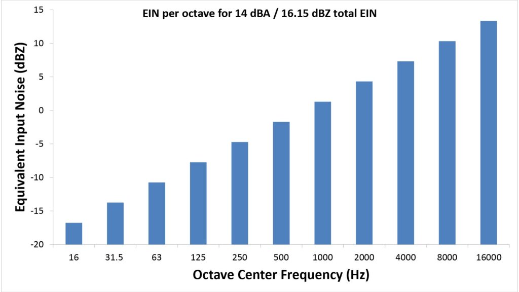
We can use the equation above to predict the EIN for any sub-band in our SINR calculations.

Doing the SINR calculations

The equations of Figure 1 and the preceding discussion should tell you everything you need to know about how to calculate the SINR. I recommend doing it in a spreadsheet, with one variable per column and one row per sub-band (if you’re calculating the SINR for multiple sub-bands). The use of a spreadsheet is particularly convenient because you can use the “goal seek” function built-into every major spreadsheet (Excel, Google Sheets, Open Office Calc, LibreOffice Calc) to find the value of a particular variable (such as microphone directivity, microphone EIN, or range) that will yield a desired minimum SINR.

Now that we’ve calculated the SINR, what do we do with it?

This purpose of this post is to introduce the SINR and describe how to calculate it. The next post in this series will address what we can do with it.

References

1. Jean-Sylvain Liénard, “Quantifying vocal effort from the shape of the one-third octave long-term-average spectrum of speech,” The Journal of the Acoustical Society of America 146, EL369 (2019). Available at https://asa.scitation.org/doi/10.1121/1.5129677 (accessed July 2022).
2. Gregory C. Tocci, “Room Noise Criteria-The State of the Art in the Year 2000,” Noise News International, Volume 8, Number 3, September 2000, pp. 106-119(14). Available at https://www.ingentaconnect.com/content/ince/nni/2000/00000008/00000003/art00001;jsessionid=6qojbt1aq4ohs.x-ic-live-02 (accessed July 2022)
3. Brad Rakerd, PhD, Eric J. Hunter, PhD, Mark Berardi, BS, and Pasquale Bottalico, PhD, “Assessing the Acoustic Characteristics of Rooms: A Tutorial with Examples,” Perspect ASHA Spec Interest Groups. 2018 January ; 3(19): 8–24. doi:10.1044/persp3.SIG19.8. Available at https://pubmed.ncbi.nlm.nih.gov/30775450/ (accessed July 2022).
4. Donald G. Albert and Stephen N. Decato, “The Pulse of a City: Noise Measurements in Baltimore,” Acoustical Society of America 159th Meeting Lay Language Papers. Available at https://acoustics.org/pressroom/httpdocs/159th/albert.htm (accessed July 2022).