Most people know that a special type of microphone is needed to pick-up sounds at long ranges. But how do such long-range microphones work—and how well do they work? Read on for detailed answers to both questions.
Why picking up sound at long ranges is hard
Before we can understand how long-range microphones work, we first need to understand the challenges involved in picking-up sound at long ranges. And to do that, we need to introduce the concept of the Signal-to-Interference-plus-Noise Ratio SINR). The SINR is a key microphone performance metric, and I have a whole series of posts on the topic:
- Predicting microphone performance—Part 1: what is SINR?
- Predicting microphone performance—Part 2: using the SINR
- Predicting microphone performance—Part 3: microphone range prediction
However, a briefer discussion of the SINR will suffice for the purposes of this post.
The Signal-to-Interference-plus-Noise Ratio (SINR)
As with receiving a faint radio signal, the challenge in picking-up sound with a long-range microphone is in ensuring that the component of the microphone’s output signal due to the desired sound is sufficiently greater than the component due to undesired sound and electrical noise. This is expressed in terms of the Signal-to-Interference-plus-Noise Ratio (SINR), in which:
- S is the sound pressure of the sound we’re trying to capture when it reaches the microphone,
- I is the interference due to ambient noise, and
- N is the sound-pressure equivalent of the microphone’s self-noise.
The SINR equation as applied to long-range pick-up
The SINR equation as applied to long-range pick-up is shown in Figure 1. It shows two microphones, one at a relatively short range R0 from the source (in this case a person speaking at conversational volume), and a second at a relatively distant range R1:
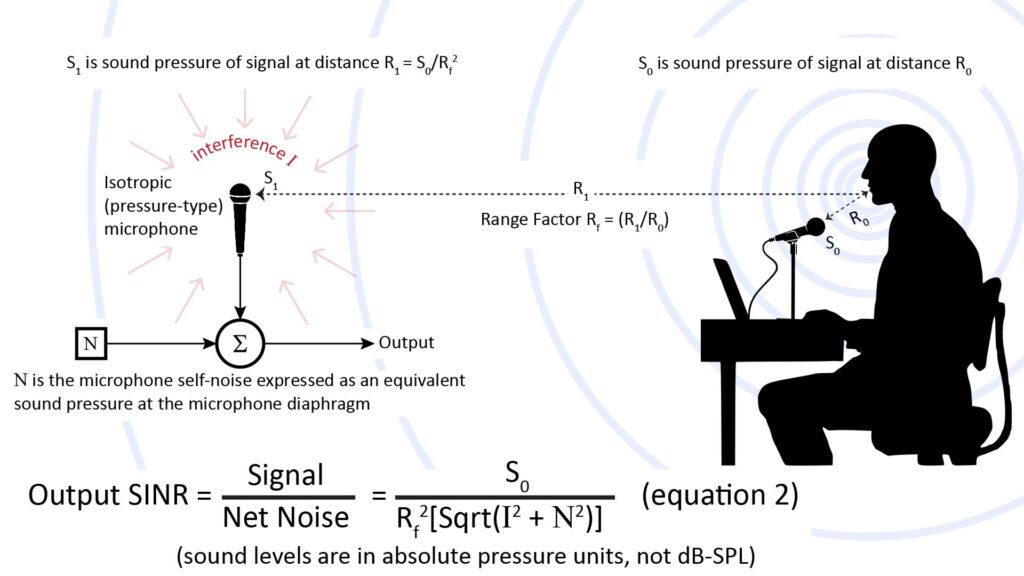
Notice that the sound pressures of equation 1 in the figure are in absolute pressure units of Pascals (Pa), rather than in Sound-Pressure Level (SPL). That’s because the denominator represents the sum of two noises, and the corresponding SPL values must first be converted into absolute pressure units before they can be added. Since an SPL value represents a ratio with respect to a reference sound pressure level of 20 μPa, we can convert between SPL and Pa as follows:
- SPL in dB = 20log(p/20 μPa), where p is the absolute pressure
- p in micro-Pascals = (20 μPa) ∗ 10^(dBSPL/20)
Note that these conversions are independent of whatever frequency weighting, if any, is used to account for the response of the human ear. For example, if an SPL value uses A-weighting, which we can write as dBA, then the corresponding absolute pressure found using the formulas above would also be A-weighted.
The SINR variables are bandwidth-dependent
Most sounds span a range of frequencies, each of which contributes to the overall sound pressure. So the values of the SINR variables depend on the assumed bandwidth: the wider the bandwidth, the greater the sound pressure.
Some of the sounds represented by the SINR variables include frequencies outside the standard 20 Hz to 20 kHz audio bandwidth. But because we can’t hear them, there is no point in including those frequencies in the SNR calculation.
In fact, it’s often useful to evaluate the SINR over a bandwidth that’s much smaller than the range of human hearing. That’s because one or more of the SINR variables can have a distinctly non-flat spectrum. In fact, this is true of long-range microphones.
When this is the case, evaluating the SINR over the whole audio bandwidth can give an inaccurate picture of the signal quality and, therefore, the pick-up range. One way to avoid this is to divide the overall bandwidth into smaller slices and evaluate the SINR in each slice. I discuss that approach in more detail in the Multiple SINRs section of my part 2 of my post on microphone SNIR.
Some typical values of the SINR variables
Now let’s discuss each of the variables of equation 1 of Figure 1 separately, assuming a bandwidth of 20 Hz to 20 kHz. When we evaluate SINR variables over the whole audio bandwidth, we need to ensure that the SPLs are A-weighted to account for the ear’s non-flat frequency response:
- The sound pressure S0 at the distance R0 from the speaker is our source sound pressure. In Figure 1 (like many long-range scenarios) the source is conversational voice, which is typically about 56 dBA (12,600 μPa) one foot away from the speaker’s mouth. I discuss voice levels and spectral characteristics in more detail in the desired sound section of Part 1 of my post on microphone SINR.
- The range factor Rf is the range extension we’re trying to achieve in our long-range scenario. It’s the range R1 to our long-range microphone divided by the range R0 at which the source sound pressure is measured. If we want a range of 100 feet and the source sound pressure is measured at 1 foot, then Rf = 100. Note that, with the variables of equation 1, Rf is equivalent to the more commonly-used term Distance Factor (DF). Later on we’ll expand equation 1 to include other variables, after which Rf will mean something a bit different than DF.
- The ambient noise pressure I at the distant microphone will vary over a huge range depending on the scenario. But 35 dBA or (1,100 μPa) is a good number for discussion purposes; it’s typical of the background level in a typical indoor setting. I have a more detailed discussion of ambient noise in the acoustic interference section of Part 1 of my post on microphone SINR.
- The microphone self-noise N, also known as the Effective Input Noise (EIN) is the electrical noise produced by the microphone itself, expressed as a fictitious sound pressure level that would cause the same noise signal at the output if the microphone were noise-free. Microphone self-noise ratings vary from about 10 dBA (63 μPa) to about 30 dBA (630 μPa). See the EIN section of my post on “The 4 key microphone specifications and why they’re important” for more information.
Now that we’ve defined the variables, let’s look at two key aspects of equation 1: the Rf2 term (which represents the propagation loss as determined by the inverse-square law) and the root-sum-squared noise term in the denominator, which is typically dominated by the ambient noise.
Propagation loss and the inverse-square law
There are several factors that could contribute to the loss experienced by propagating sound. But the overwhelming factor, and the only one we need to consider for long-range sound pick up, is the inverse-square loss. That loss is given by the inverse-square law.
As was shown in Figure 1, sound from the speaker’s mouth propagates outward as a spherical wavefront. Since the area of a sphere is proportional to the radius squared, the inverse-square law says that, for sound propagating in a free-field, the sound pressure decreases with the square of the distance to the source. Thus, the SPL produced by a source will drop by a factor of 4 (equivalent to -6 dB) for every doubling of the range.
For example, if the sound pressure one foot away from a person’s mouth is 56 dBA, then it will be 50 dBA at two feet, 44 dBA at four feet, 38 dBA at eight feet, and so on. The following chart shows the inverse-square loss as a function of the range factor, which we previously define as the ratio of the range to the baseline range at which the source sound pressure was measured:
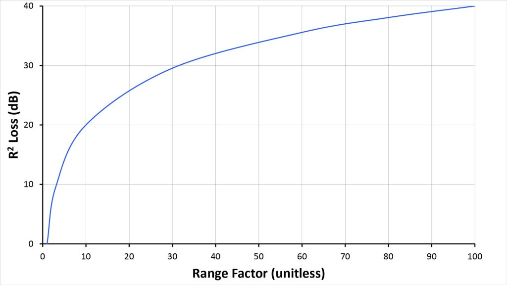
So, for example, increasing the range from one foot to six feet — a range factor of 6 — would decrease the SPL of the source by about 16 dB, or a factor of 6.3. That’s a significant loss, and only at six feet. At 100 feet, the range factor is 100 and the loss increases to 40 dB, or a factor of 10,000. That’s a huge deficit to overcome.
Are there conditions under which the inverse-square law doesn’t apply?
The inverse-square law doesn’t apply at distances less than a wavelength or so from a sound-source, but that’s obviously not relevant to a long-range scenario.
However, there is a phenomenon that can mitigate the inverse-square loss in a long-range scenario: ducting.
As the name implies, ducting is a phenomenon in which propagating sound waves are constrained in at least one dimension from spreading outward. Significant ducting can occur in an outdoor scenario when the air temperature is warmer than the ground (such as shortly after sunrise, especially when the ground is snow-covered). This causes a temperature gradient (known as a thermocline) which tends to refract sound downward, toward the ground. Sound emitted by a source near the ground will then bounce between the thermocline and the ground as it propagates horizontally, so that the sound pressure level drops off approximately linearly with distance rather than as the square of the distance.
Obviously, ducting can significantly increase the maximum range of a long-range microphone. However, we obviously can’t rely on ducting, so I’m not going to consider it further in this post.
Ambient noise typically dominates total noise when picking-up sound at long ranges
The second term in the denominator of the SNR equation 1 of Figure 1 is the total acoustic noise power at the microphone. This includes two components: the ambient noise I and the microphone self-noise N.
Because noise signals are random and independent, they don’t add coherently as voltages, but rather add incoherently as powers. So the sound pressure of the sum of the ambient noise and self-noise isn’t equal to the sum of the pressures, but rather to the Root-Sum-Squared (RSS) of the pressures: Ntotal = sqrt(I2 + N2).
Earlier in this discussion, we mentioned 35 dBA as a typical indoor ambient noise level and a range of 10 to about 30 dBA for microphone equivalent self-noise. A microphone self-noise of 30 dBA is very high, and even inexpensive Electret Condenser Microphone (ECM) capsules offer self-noise specs of 20 dBA or better.
So let’s assume an ambient noise of 35 dBA and a self-noise of 20 dBA. To find the total noise, we have to first convert these values to absolute pressure units (as described earlier in this post) and take their RSS. If we then convert the total noise back to dBA, we get 35.1 dBA…which means that the microphone self-noise has a negligible impact on the total noise.
In fact, if the either the ambient noise or the self-noise is significantly larger than the other quantity, it will dominate the total noise. Only when the two quantities are comparable do both have a significant effect. This is illustrated in Figure 2, which plots the total noise versus ambient noise for three values of microphone self-noise:
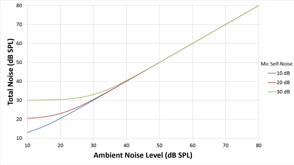
We can see that, at our assumed ambient noise level of 35 dBA, we can safely ignore microphone self-noise. However, microphone self-noise can become an issue in some circumstances, as we’ll see later.
Required SINR for picking-up voice
Now we know how to calculate the SINR in a typical long-range pick-up scenario, but how much SINR do we need? That depends on what we intend to do with the captured sound.
If we want extremely high fidelity, we might shoot for a SINR approaching 80 dB. However, such a SINR is possible only in a soundproof recording booth using a low-noise microphone placed within a few inches of the source. And we don’t need an SINR of 80 dB for great sound quality. For example, Shure says that “If speech level is 30dB to 50dB above background noise level, intelligibility will be good to excellent” [1].
At the other extreme, in a surveillance application we might only need a SINR just barely enough to understand speech. Wikipedia [2] cites 12 dB as the SINR threshold for 100% speech intelligibility, while Studebaker and Sherbecoe [3] obtained intelligibility scores approaching 100% at a SINR of 8 dB.
So a minimum required SINR of 8 dB is probably a reasonable assumption if we’re interested in the absolute maximum range in a surveillance or sports application.
What about the “Cocktail Party Effect”?
You might have heard about the “Cocktail Party Effect,” which refers to the ability of the human auditory and neural systems to isolate and understand speech from a single talker in the presence of noise from many competing talkers. When the Cocktail Party Effect is operative, speech can be understandable at SINR’s even less than 0 dB.
However, the Cocktail Party Effect happens only in person, because it apparently involves processing of amplitude and phase information from both ears. So, unfortunately, we can’t count on the Cocktail Party Effect in establishing the minimum required SINR for sound captured by a microphone.
Putting it all together: estimating the range of an ordinary microphone
Now that we’ve established a minimum required SINR, we can determine the maximum achievable range factor with the ordinary microphone shown in Figure 1.
There are two ways to do this: the accurate way, and the easy way:
- The accurate way is to rearrange equation 2 of Figure 1 to solve for Rf as a function of the other variables.
- The easy way is to assume that the microphone self-noise is dwarfed by the ambient noise (which, as previously discussed, is usually a pretty good assumption) to simplify the calculation.
Here’s an example of the easy way.
With a required SINR of 8 dB and an ambient noise level of 35 dBA, we would need a signal level S1 of 43 dBA at the microphone diaphragm. If the sound we want to pick up is conversational speech (which has a typical level of 56 dBA at one foot from the speaker’s mouth), then we can tolerate an inverse-square loss of 13 dB. Looking at Figure 2, we can see that a 13 dB inverse-square loss corresponds to a range factor of about five. However, we can get a more exact estimate using the following equation:
- RF = 10^(L/20), where L is the allowable inverse-square loss in SINR. (equation 2)
According to this equation, an inverse-square loss of 13 dB corresponds to a range factor of 4.5. So the maximum pick-up range in this example is just 4.5 feet…and that’s just for barely intelligible voice!
Suppose we want higher-quality sound, say with an SINR of 16 dB. Then we’d need a signal level of 51 dBA at the microphone, allowing a 5 dB inverse-square loss. Per equation 2, a 5 dB inverse-square loss translates to range factor of 1.8. So the maximum pick-up range is now just 1.8 feet.
Now that we understand the two big challenges in long-range pickup—the inverse-square loss and ambient noise—we can investigate ways to overcome them.
The keys to increased microphone range: directivity and gain
From the SINR equation in Figure 1 and the discussion above, it’s obvious that we can’t increase the pick-up range by simply amplifying the microphone output, because that would amplify the noise as well as the signal (and therefore wouldn’t increase the SINR). And we can’t just use a microphone with lower self-noise because, as shown in Figure 3, ambient noise usually dominates the overall noise.
Instead, the only way to significantly increase the pick-up range in a typical scenario is to reduce the ambient noise, and—after we’ve reduced it sufficiently that self-noise becomes an issue—to optionally reduce the effects of self-noise.
Reducing the effects of ambient noise via directivity
If all of the ambient noise happens to be coming from the same direction as the sound we’re trying to capture, then there’s really no way to reduce it (well, if we’re really lucky, the noise will be limited to a narrow range of frequencies that we can filter-out without affecting the signal fidelity, but that’s rarely the case).
Fortunately, at least some of the ambient noise will almost always come from a different direction than the target sound. In fact, ambient noise is often nearly isotropic, meaning that its power is nearly uniform with direction.
If at least some of the ambient noise is coming from a different direction than the target sound, then we can reduce it by making the microphone directional.
The term used to describe the degree to which a microphone is directional is directivity. A microphone’s directivity (D) is defined as the ratio of its peak sensitivity to its sensitivity averaged over all directions. It’s sometimes also in expressed in dB as the Directivity Index (DI).
A microphone with an isotropic polar pattern therefore has a D of 1 and a DI of 0 dB, since it’s equally sensitive in all directions. A microphone with a hypercardioid pattern—which is the most directive pattern achievable with an ordinary studio microphone—has a D of 4 and a DI of 6 dB. See the Polar Response section of my post on the 4 key microphone specifications for much more information on microphone polar patterns.
If the ambient noise is isotropic, as it usually is, then the total noise is reduced almost one-for-one by the DI. For example, using a hypercardioid mic instead of an isotropic mic will reduce the ambient noise by 6 dB.
The Distance Factor (DF)
Even if we use directivity to reduce the effects ambient noise, the ambient noise term will often still dominate the denominator of the SINR. In that case, the effects of microphone self-noise can be ignored, and the increase in pick-up range can be approximated by a very simple metric known as the Distance Factor (DF).
A directional microphone’s DF is the increase in range (over an isotropic microphone) provided by its directivity; it’s the range factor at which the additional inverse-square loss of the desired sound is exactly compensated by the reduction in isotropic ambient noise. The DF is found using the following equations:
- DF = Sqrt(D), where D is the Directivity, or
- DF = 10^(DI/20), where DI is the Directivity Index in dB.
However, the DF has significant limitations in predicting microphone range, as I’ll explain later.
Reducing the effects of self-noise via acoustic gain
With an ordinary studio microphone, the ambient noise level usually dwarfs the microphone self-noise. But in long-range microphones, the directivity can be high enough to knock-down the ambient noise level to the point where the self-noise rivals it.
In that case, further increases in range are possible by reducing the effects of the self-noise. We can do this via acoustic gain, which increases the sound pressure that reaches the microphone diaphragm(s).
Including microphone directivity and gain in the SINR equation
We can update the diagram and SINR equation of Figure 1 to consider the use of a long-range microphone, instead of an isotropic microphone, at the remote pick-up location. The result is shown in Figure 4:
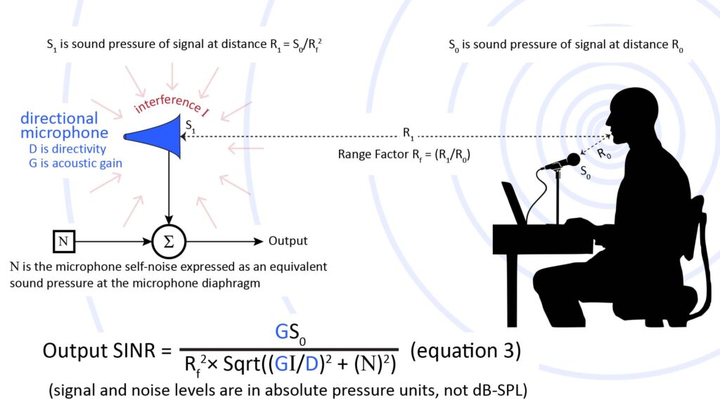
Figure 4 shows a directional microphone that has a directivity D and a gain G.
- The directivity D is as previously described: it’s the linear (non-dB) form of the Directivity Index (DI).
- The gain G is a linear multiplier on the sound pressure reaching the microphone diaphragm.
We can see from Figure 4 that the directivity D directly reduces the interference due to ambient noise. On the other hand, the gain G increases both the signal and interference terms by the same amount (and therefore doesn’t mitigate ambient noise), and thereby reduces the influence of the microphone self-noise N.
We’ve already seen that, with an ordinary microphone, ambient noise usually dwarfs the self-noise. But with long-range microphones, D can knock the ambient noise level down to where the self-noise starts to rival it—and that’s when gain can increase the pick-up range.
We could easily re-arrange equation 3 of Figure 4 to express Rf as a function of the other variables. However, there’s a catch.
The catch: directivity and gain are usually frequency-dependent
While directivity and gain are the keys to long-range pick-up, they have one big issue. As we’ll see below, the high directivity provided by long-range microphones—and the acoustic gain for those microphones that provide it—depend on their physical size in wavelengths.
This has two important implications.
Long-range microphones aren’t practical for capturing low frequencies
The frequency dependence of gain and directivity means that the lower the lowest frequency of interest, the larger the microphone must be to achieve a given range. Specifically, at least one physical dimension of the microphone must be comparable to the wavelength at the lowest frequency of interest in order to achieve significant range extension.
The required size usually isn’t an issue for capturing relatively high-frequency sounds (such as some bird or bat vocalizations), but can be an issue for capturing human voice at long ranges—and is most definitely a major issue for capturing high-fidelity music.
In fact, a microphone capable of picking-up high-fidelity music at long ranges would be impractically huge; it would need to be at least 10 feet long or wide to achieve significant range extension at bass frequencies.
On the other hand, substantial ranges are possible with a reasonably-sized device when capturing human voice. That’s because voice remains intelligible even without some of its lower frequencies.
The voice bandwidth: fidelity vs intelligibility
The full bandwidth of human voice extends over a large fraction of the entire audible range—from around 100 Hz to around 10kHz. Microphones intended for high-fidelity voice capture have useful bandwidths that extend over at least this range. By the way, I discuss microphone bandwidth requirements for both voice and music in detail in the Effective Bandwidth section of my post on the 4 key microphone specifications.
However, voice is still intelligible when it is limited to a smaller bandwidth, such as by passing it through a bandpass filter. In fact, the original analog telephone system supported a bandwidth of only 300 Hz to 3 kHz. So, if a long-range microphone provides the required directivity and gain down to around 300 Hz, we can be sure that the voice it captures will be fully understandable.
However, the wavelength at 300 Hz is about four feet, so obtaining significant directivity down to 300 Hz would still require an impractically large device. Fortunately, speech remains intelligible even when the low-frequency cut-off is raised above 300 Hz.
One of the seminal studies on the intelligibility of band-limited speech was undertaken by Studebaker and Sherbecoe [3]. Figure 5 is based on data from that study, and plots the intelligibility of high-pass-filtered speech at a signal-to-noise ratio of 8 dB as a function of the high-pass cutoff frequency. The intelligibility is given in terms of W-22 “percentage intelligibility” scores (the W-22 score is a speech intelligibility metric developed by the Central Institute for the Deaf):
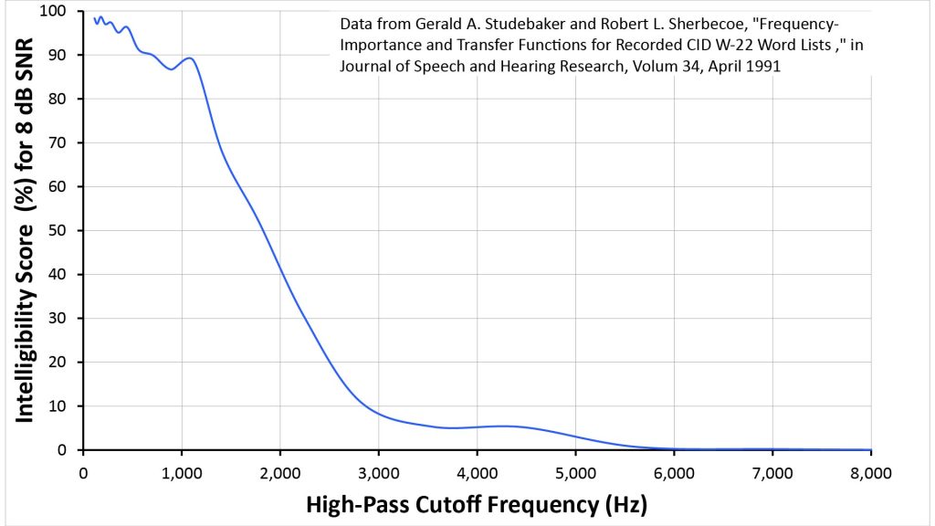
This plot shows that intelligibility remains above 85 percent even when the speech is high-pass filtered with a cutoff of 1 kHz. We can infer from this that speech will be mostly intelligible when captured by a long-range microphone that provides adequate gain and directivity down to 1 kHz.
Even better, the high-pass filter used to obtain the data above had a sharpness of 48 dB per octave, whereas the low-frequency roll-off in directivity and gain for long-range microphones can be much shallower (in fact, it’s just 6 dB per octave for parabolic mics). So, even if a long-range microphone doesn’t provide the full required directivity or gain at lower frequencies, it might still work well enough at those lower frequencies to contribute significantly to the overall intelligibility.
Of course, speech intelligibility isn’t the same thing as speech fidelity. If we want the speech to sound good, then our microphone must have at least some sensitivity down to 300 Hz (or preferably even lower), so that we can apply electronic equalization to flatten the response.
The frequency dependence affects the range prediction
The second issue with the frequency dependence of directivity and gain is that it affects the way we predict the range of long-range microphones.
That’s because it causes the SINR to vary much more with frequency than with a conventional microphone used for short-range pick-up.
That, in turn, means that we cannot use a single SINR calculation evaluated over the whole audio bandwidth (as in the previous examples) to accurately predict the achievable range.
Fortunately, there are three methods to address the frequency-dependence of directivity and gain in order to predict the range of long-range microphones; I discuss them in detail in Predicting microphone performance—Part 3: microphone range prediction. Here’s a brief summary:
- We can break-up the voice bandwidth into multiple narrow sub-bands, evaluate the SINR over each sub-band, and then predict the overall range using a function of the multiple SINR values. This is the most accurate but also the most complex method.
- We can base the range prediction on the SINR evaluated over a narrow sub-band centered at 2 kHz. This is less accurate than the multiple-SINR method, but also simpler because it enables a closed-form solution of equation 3 for the range extension. It also has the advantage of comprehending the effects of gain and microphone self-noise.
- If we neglect the effects of microphone self-noise, we can skip equation 3 completely and instead base the range prediction on the Distance Factor at 2 kHz. This is the least accurate method but still gives a useful rough approximation of the achievable range.
All of the range predictions in this post are based on the multiple-SINR method (method 1 above).
Types of long-range microphones
Now that we understand the challenge of long-range pick-up and how it can be met through directivity and gain, we’re finally ready to discuss how the various types of long-range microphones actually work.
There are four main types of microphone that are capable of picking up sound at longer ranges than a conventional hypercardioid studio microphone:
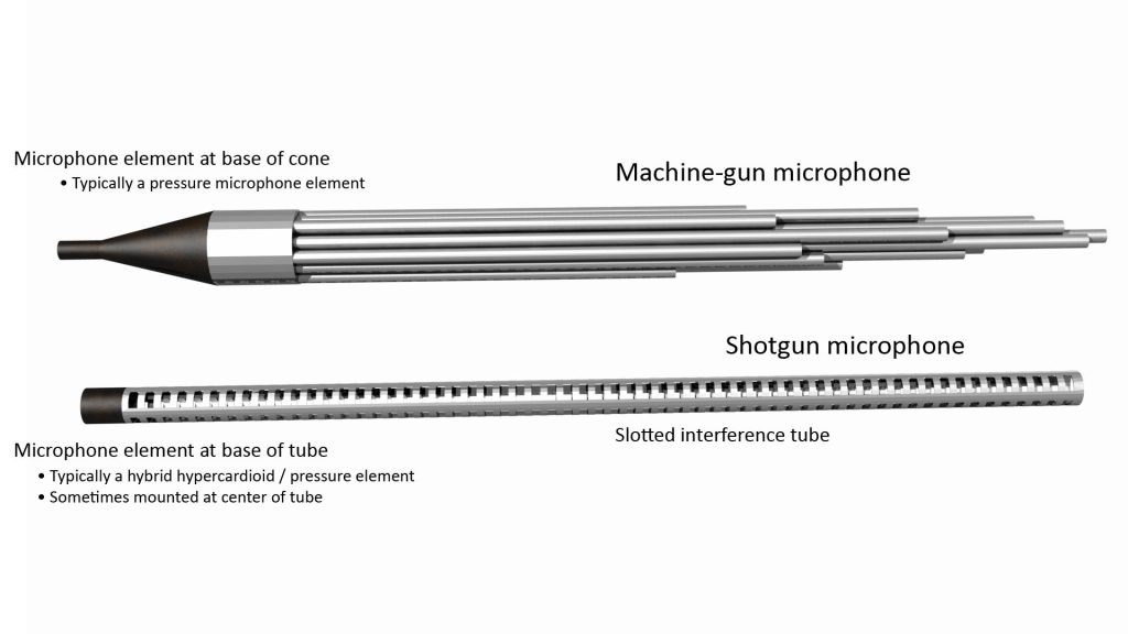
- Shotgun microphones are a form of line microphone, which consist of a microphone element acoustically coupled to an array of sound-receiving ports arranged along a line. The line of ports (which constitutes the sound-collection aperture) has minimal effect on on-axis sound, but causes destructive interference of off-axis sound. The ports can consist of slots in an interference tube (as in modern shotgun microphones), or the open ends of a cluster of tubes of varying length (as in now-obsolete machine-gun microphones). See my detailed post on how shotgun microphones work for a deep-dive into shotgun microphone principles and performance.
- Parabolic microphones are “sound spotlights” that use a parabolic reflector (or “dish”) to focus on-axis sound on a microphone element. Obviously, the mouth of the dish provides a large sound-collecting aperture, and the coupling to the microphone element occurs by reflection from the dish’s interior surface. See the complete guide to parabolic microphones for more on their principles of operation what you need to know before building or buying one.
- Horn microphones work a like a megaphone in reverse: they amplify on-axis sound by funneling it from a wide mouth to a microphone element mounted in a narrow throat. The horn’s wide mouth forms the sound-collecting aperture, while the horn’s body acts as an acoustical transformer to couple the captured sound to the microphone diaphragm. Check out my post on how horn microphones work if you want to know the gory details.
- Array microphones use multiple microphone elements whose outputs are electronically processed to yield the array output. The effective sound-collecting aperture is then the area that encompasses the microphones. Of course, I have a detailed post on how array microphones work, too.
The following table and paragraphs summarize the high points for each of these types of microphone; again, see the detailed posts mentioned above for much information.
| Shotgun (interference tube or machine-gun tube-cluster only) | Parabolic | Array | Horn | |
| Directivity D (linear, not dB) | D≈4L/λ, where L is interference tube length and λ is wavelength | D≈ε(πd/λ)2, where ε is an efficiency factor that ranges from 0.5 to 0.7, d is dish diameter, and λ is wavelength | D=2Ns/λ for broadside array and D=4Ns/λ for end-fire array, where N is number of elements, s is element spacing, and λ is wavelength | Comparable to parabolic dish of same area as horn mouth at lower frequencies; less than comparably-sized dish at higher frequencies (depends on horn shape) |
| Gain G | G≈1.0 | G≈D | G≈N, where N is number of elements | G≈ratio of mouth to throat areas for Acoustic Pressure Horn; G≈ratio of mouth to throat radii for Acoustic Velocity Horn |
| On-axis frequency response | Flat | Low-frequency roll-off, per D and G | Either flat or with low-frequency roll-off, depending on type of array. See array microphone post. | Either mostly flat or with low-frequency roll-off, depending on type of horn. See horn microphone post. |
Shotgun microphones (and line microphones in general)
The shotgun mic is the conventional go-to microphone for picking-up sound at ranges a bit further than possible with conventional studio microphones.
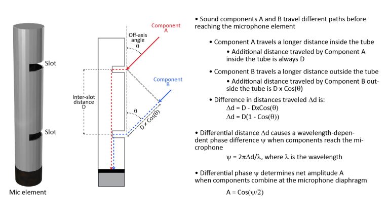
The shotgun microphone is the most widely-used type of line microphone, in which sound reaches a microphone element via multiple ports arranged along a line. The ports break up incident sound into separate components which recombine at the microphone element. For on-axis sound, the components reach the microphone in-phase, so they recombine constructively. However, for off-axis sound, the components arrive at the microphone element with different phases, whereby they partially cancel through destructive interference.
In the first line microphones (known as Gatling-gun or machine-gun microphones), the ports were the open ends of a cluster of tubes of varying length. In the modern shotgun microphone, the ports are holes or slots in the sidewall of a single interference tube (optionally, the front end of the interference tube itself is also open, providing another port, and the interference tube may be mounted concentrically within another tube).
Shotgun microphone operation is discussed in detail in my post on how shotgun microphones work, but here are some highlights (which apply to all types of line microphone, not just shotgun microphones:
- Unlike the other types of directional microphone on our list, a shotgun microphone provides no gain, so gain G is approximately 1.0.
- A shotgun microphone’s length determines its directivity (which, like all microphones, will be frequency-dependent). Therefore, the longer the desired range, the longer the required shotgun microphone.
- A shotgun microphone’s length also determines the lowest frequency at which it can provide useful directivity. Specifically, a shotgun microphone should be no less than a half-wavelength long at the lowest frequency at which off-axis rejection is desired. So, even if the required range is just a couple of feet, a long shotgun microphone might be needed if the ambient noise has a significant low-frequency component, such as with room echoes. A work-around to this limitation, which almost all modern shotgun microphones use, is to combine the shotgun microphone’s interference tube with a conventional hypercardioid microphone configuration; the hypercardioid provides modest directivity at low frequencies, while the interference tube provides high directivity at higher frequencies. Note that Table 1, the performance characteristics listed for the shotgun microphone are for the interference tube or tube-cluster only, and don’t include the effects of any integrated low-frequency hypercardioid capability.
- Unlike some of the other directional microphone on our list, a well-designed shotgun microphone can provide a reasonably flat on-axis frequency response without equalization.
The useful range of a shotgun microphone depends on the ambient noise level and spectrum, but is only a few feet at most. And a good shotgun microphones is also quite expensive…unless you build it yourself. Of course, I have a post on that in the works.
Parabolic microphones
Thanks to the televised sporting events (primarily American football), the parabolic microphone is the type of microphone most commonly associated with very long ranges. It’s also the go-to microphone for surveillance applications (for both human and animal subjects).
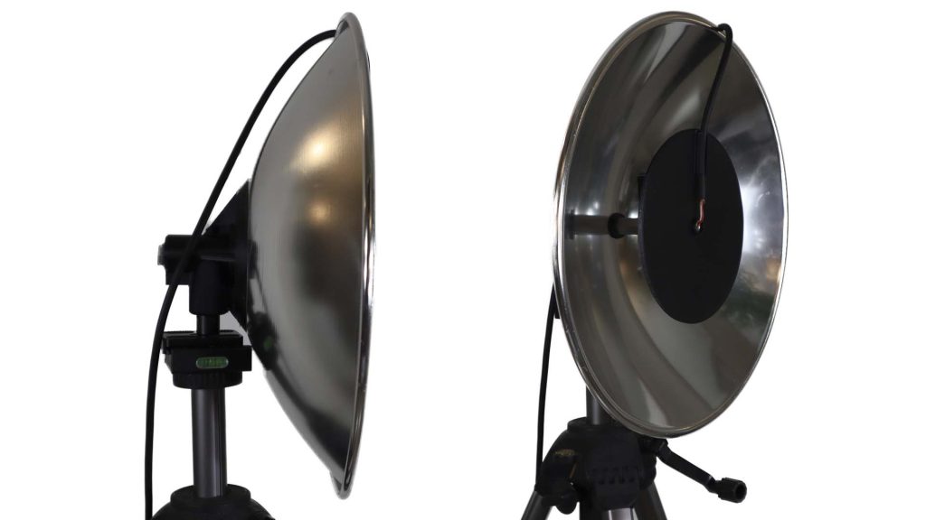
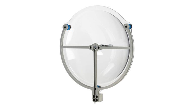
As shown in Figure 9, a parabolic reflector (or “dish”) has the property that a sound wave striking it from the on-axis direction—regardless of where on the dish it strikes—will be reflected to a specific focal point determined by the shape of the dish.
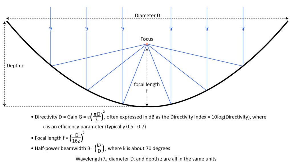
Therefore, if a microphone element is mounted at that focal point, it will receive all of the acoustic power received by the entire dish, which can result in significant acoustic gain. And sounds arriving from off-axis won’t experience this gain, which is what gives a parabolic reflector its high directivity.
Parabolic microphone operation is discussed in detail in my post on the complete guide to parabolic microphones, but here are some highlights:
- A parabolic dish can provide both high directivity D and gain G, with both being proportional to the square of the dish diameter in wavelengths.
- For voice capture, the minimum required dish diameter for a useful parabolic microphone is about 8 inches. With a dish this size, voice can be captured with full intelligibility up to about six feet, and with marginal fidelity up to about 12 feet, in typical conditions. Higher frequency sounds (such as bird calls) can be captured much further. In fact, a parabolic mic is the most cost-effective way to capture high-frequency sounds at long range.
- Larger dishes, of course, will provide greater range. All other things being equal, range scales approximately with the dish diameter. The most common diameter for a parabolic dish is about 2 feet, which will have triple the ranges mentioned above for the 8 inch dish.
- The gain of a parabolic microphone decreases with decreasing frequency, so the output has a low-frequency roll-off of 6 dB per octave. Therefore, if used to capture voice, the output can and should be equalized to cut the higher frequencies.
- For best results, the dish must be truly parabolic. Some DIY projects suggest repurposing items such as mixing bowls or trash-can lids to provide acoustic gain for long-range microphones, and while such items will generally provide some gain, it will be far less than what a genuine parabolic reflector would provide.
- It’s critical that the diaphragm of the microphone element be accurately positioned at the dish’s focal point. This is much harder to do than it might seem from some online DIY projects.
Array microphones
An obvious way to increase the sound-capture area of a microphone would be to just increase the area of the microphone’s diaphragm. Unfortunately, this would also increase the diaphragm’s mass, reducing the microphone’s high-frequency response. However, the same effect can be achieved by using an array of microphones and processing their outputs in various ways.
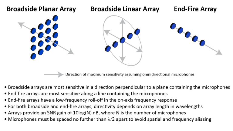
Array microphones can be configured in four main ways, as shown in Figure 10:
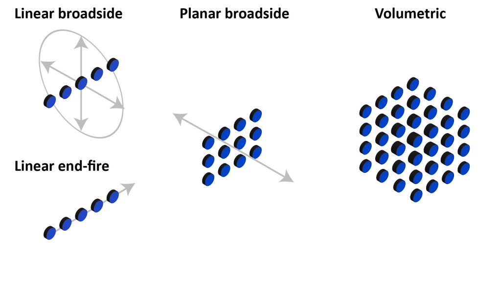
Array microphones are based on the same principles used by all directional microphones, except that the destructive interference which suppresses off-axis sound occurs in the electrical domain in an array microphone, rather than in the acoustic domain as with other types of directional microphone.
Array microphones are discussed in more detail in my post on how array microphones work, but here are some highlights:
- There are many classes of array microphone, depending on how the microphone elements are physically arranged and how their outputs are processed to yield the overall array output. In general, you can design an array microphone to have either a flat on-axis frequency response or a polar pattern that retains its shape over a wide frequency range, but not both.
- The directivity of an array microphone depends on the product of the number of elements and the element spacing in wavelengths. In other words, the directivity depends on the length or area of the array’s aperture in wavelengths: the bigger the aperture, the greater the directivity.
- However, the elements must be spaced no further than a half-wavelength or a quarter-wavelength apart (depending on the type of array) at the highest frequency of interest, in order to avoid aliasing in the polar pattern or frequency response.
- The upshot of the above two facts is that an array microphone that provides both high directivity at low frequencies (which requires a large aperture) and a wide frequency response (which requires a small spacing) can require a lot of microphone elements. For example, an array that provides the same directivity as a 24-inch parabolic dish, and yet is capable of a flat frequency response up to 8 kHz, would require about 850 microphone elements. So array microphones are much less cost-effective than other types of directional microphone when high directivity and a wide bandwidth is required.
- On the other hand, arrays can be extremely practical in applications that can do without either high directivity or wide bandwith:
- If limited bandwidth and a low-frequency roll-off can be tolerated, then a modest but useful directivity of four (6 dB) can be achieved with just a two-element array. In fact, cardioid and hypercardioid studio microphones are based on the same principles as two-element differential arrays.
- If directivity isn’t important but high fidelity is, then a small array can be used to obtain a flat frequency response with extremely low self-noise. That’s because the self-noise of certain arrays decreases with the number of elements, so an array of ten elements will have a self-noise that is 10 dB lower than each individual element.
For these reasons, array microphones on their own are generally not the best choice for long-range applications. However, a hybrid design that combines a microphone array with one of the other directivity enhancing approaches of Table 1 can be quite advantageous.
Horn microphones
The basic principle of a horn microphone is straightforward: sound arriving at the mouth of a horn is concentrated at its throat, where the concentrated sound is sensed by a microphone element. This concentration effect provides acoustic gain, while the large mouth area provides wavelength-dependent directivity.
As shown in Figure 11, there are two kinds of horn microphone: the Acoustic-Pressure Horn (APH) microphone and the Acoustic-Velocity Horn (AVH) microphone. An APH has a sealed throat and uses a pressure microphone element, while an AVH has an open throat and uses a velocity-sensing microphone element (also known as a pressure gradient microphone element):
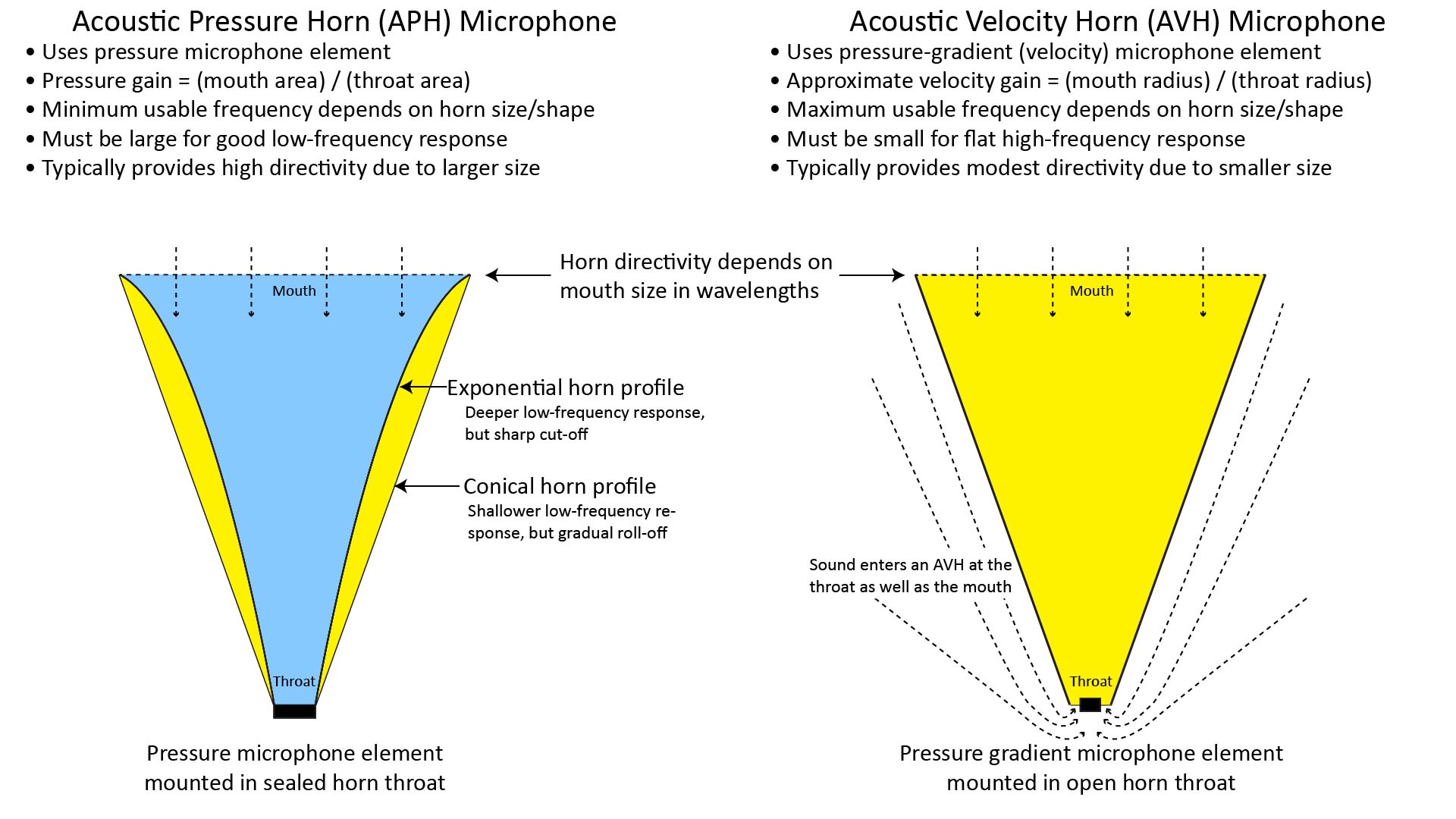
Horn microphones are discussed in more detail in my post on how horn microphones work, but here are some highlights:
- As with parabolic microphones, horn microphones provide both directivity and gain.
- As with parabolic microphones, the directivity of a horn microphone is wavelength-dependent and determined by the dimensions of its mouth. Parabolic dishes and horns having the same mouth area will have roughly the same directivity at wavelengths comparable to the mouth width, but a horn’s effective width decreases at shorter wavelengths in a way that depends on the type of horn.
- The gain of a horn microphone is the product of two factors:
- a pressure gain (in the case of an APH) or a velocity gain (in the case of an AVH), and
- an efficiency factor that reflects how well sound is coupled from the horn’s mouth to its throat.
- The pressure or velocity gain of a horn mic is independent of wavelength and depends only on the ratio of the size of the mouth to the size of the throat. In an APH, the pressure gain is the ratio of the areas of the mouth to the throat, while in an AVH, the velocity gain is approximately the ratio of the radii of the mouth to the throat.
- In an APH, the efficiency with which sound is coupled from the mouth to the throat is wavelength-dependent and decreases with decreasing frequency. So, all APHs behave like high-pass filters, and achieving a deep low-frequency response with an APH requires a large horn. The shape of the efficiency-versus-frequency curve is determined by the shape of the horn. A conical horn (like a megaphone) has a relatively high low-frequency cutoff for its size, but its response rolls-off smoothly below the cutoff. On the other hand an exponential horn has a lower low-frequency cutoff for the same size, but the response drops sharply below the cutoff. There are other horn shapes (such as parabolic and hyperbolic) with different efficiency-versus-frequency curves.
- In an AVH, on the other hand, the coupling efficiency is not wavelength dependent. So, even a small AVH can achieve good low-frequency response. However, the pressure-gradient elements used in an AVH have lower sensitivity than the pressure elements used in an APH, and the velocity gain provided by an AVH is smaller than the pressure gain provided by an APH of comparable size. For this reason, an AVH is probably not a good choice for long-range voice pickup, but it offers some unique advantages for shorter-range pickup and when low-frequency response is critical.
- Horn microphones do have one unique disadvantage: the air mass inside a horn resonates at a fundamental frequency (and harmonics thereof) determined by the size of the horn. Depending on the horn design, the amplitude of the resonance can be negligible, or it can be high enough to cause audible ripples in the horn’s frequency response.
- Horn microphones are easier to build than other types of long-range microphones. Effective horn microphones can be built using a variety of devices such as hand-rolled conical horns, horn “waveguides” manufactured for use in speakers, and even adapted cheerleading megaphones.
- In general, the pick-up range of a horn microphone will be greater than that of a shotgun microphone of comparable length, but less than that of a parabolic microphone of comparable volume.
How well do long-range microphones really work?
While Table 1 summarized the key attributes of the various types of long-range microphones, we can get an even better idea of their relative capabilities with performance projections for some examples of each type.
Choosing the long-range microphones for comparison
One way of ensuring an apples-to-apples comparison between various types of long-range microphones would be to select examples that share the same cost, volume, weight, or some other key attribute.
But a more useful approach might be to select typical examples of each type…examples of what you’re likely to find in the marketplace (or build, if you’re a DIYer). That’s the approach I’ve decided to use for this discussion. Table 2 lists the examples we’ll compare:
| Type | Description | Notes |
| Parabolic | 12-inch dish with dish efficiency of 0.6 | Typical size of a DIY parabolic microphone using a solar-cooker dish |
| Parabolic | 26-inch dish with dish efficiency of 0.6 | Typical of commercially-available parabolic microphones; largest parabolic mic that isn’t prohibitively difficult to handle |
| Shotgun | 12-inch interference tube with hypercardioid element | Typical of modern long shotgun mics (such as the Shure VP89L) which use a hybrid hypercardioid/interference-tube arrangement |
| Shotgun | 24-inch interference tube with pressure mic element | Typical of a long DIY shotgun or machine-gun mic that isn’t prohibitively difficult to handle and does not include a hypercardioid element |
| Array | 16-element array with 0.33-inch spacing | Represents the largest DIY array mic (in terms of number of elements) that’s still relatively easy to build |
| Horn | 12-inch exponential Acoustic Pressure Horn (APH) | Small DIY horn microphone using an inexpensive off-the-shelf speaker horn |
| Horn | 32-inch conical Acoustic Pressure Horn (APH) | Large DIY horn microphone using an off-the-shelf cheerleader’s megaphone; |
Of course, this list isn’t intended to be exhaustive, but rather just to illustrate the differences between typical examples of each type of microphone.
To ensure an apples-to-apples comparison of the various sound-collecting approaches, we’re going to assume the same microphone element self-noise of 14 dBA for all of the mics of Table 2.
Directivity and gain of typical long-range microphones
The ultimate measure of a long-range microphone’s capability is its maximum pick-up range, but first we’re going to look at two performance attributes that help determine the maximum range:
- Directivity versus frequency. As we’ve already discussed, directivity is the key attribute of a long-range microphone, and directivity is frequency-dependent. So, one important criterion for evaluating a long-range microphone is its directivity versus frequency curve.
- Gain versus frequency. As previously discussed, acoustic gain can help increase a microphone’s range, and a frequency-dependent gain will affect a microphone’s frequency response.
Directivity versus frequency of typical long-range microphones
Estimating directivity versus frequency is straightforward for all four types of directional microphone except the horn; the basic equations were listed previously in Table 1. For more background, see my detailed posts on each type of microphone.
Figure 12 shows the estimated directivity versus frequency for the microphones of Table 2.
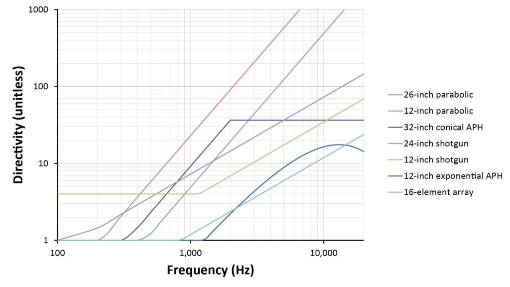
We can make at least five observations from the curves of Figure 12:
- The only microphone that provides significant directivity at frequencies below 400 Hz is the 12-inch shotgun microphone. But that’s because this particular shotgun mic (like all the commercial shotgun mics available today) is a hybrid microphone that uses a hypercardioid capsule at low frequencies and the interference tube at higher frequencies. So all of the of the low-frequency directivity is due to the hypercardioid capsule, rather than the shotgun mic’s distinctive interference tube. None of the other mics we’re comparing in this discussion use a hybrid arrangement that incorporates a hypercardioid capsule, but they could.
- The 26-inch parabolic dish provides the greatest directivity at voice frequencies, which is consistent with the fact that it has the largest sound-collecting aperture.
- The directivity of the parabolic dishes rises monotonically at 6 dB per octave with increasing frequency, reaching very high values at higher frequencies. But high directivity above several kHz is of limited value in a voice application, because (as previously shown in Figure 5) its the frequencies between 1 and 3 kHz that contribute most to voice intelligibility.
- The directivity of the horn microphones also initially rises at 6 dB per octave with increasing frequency, but then either flattens out (for the conical APHs) or actually decreases at higher frequencies (for the exponential APHs). As long as the directivity peaks at around 2 kHz, such a directivity-versus-frequency curve is fine for voice.
- The smaller microphones (the 16-element additive broadside array and the small AVH) provide relatively little directivity even at high frequencies.
Gain versus frequency of typical long-range microphones
As with directivity, estimating gain versus frequency is straightforward for all four types of directional microphone except the horn; the basic equations were listed previously in Table 1. For more background, see my detailed posts on each type of microphone.
Figure 13 shows the predicted gain versus frequency of the mics of Table 2.
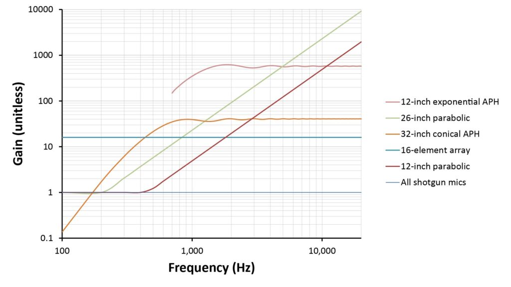
We can make at least four observations from the curves of Figure 13:
- Shotgun microphones provide no acoustic gain.
- The 16-element additive broadside array provides a flat frequency response with significant gain.
- The 12-inch exponential Acoustic Pressure Horn (APH) provides the highest gain in the heart of the voice bandwidth, but its response cuts-off abruptly below about 700 Hz. So we can’t apply electronic equalization to boost those lower frequencies.
- The 32-inch conical APH provides less gain than the much smaller exponential APH used in this example (that’s because this cheerleader’s megaphone on which this APH is based has a relatively wide throat). However, the conical APH doesn’t have an abrupt low-frequency cutoff like the exponential APH, so its output can be equalized to flatten the response.
- The frequency response curves of the parabolic dishes have the same shapes as their directivity curves: they rise monotonically with frequency at 6 dB per octave. So, as with the APH microphones, their outputs need to be equalized for the best sound quality.
Maximum range of typical long-range microphones
The ultimate measure of the performance a long-range microphone is its pick-up range. As I’ve already described, the increased range provided by long-range microphones is due to their directivity and (optionally) acoustic gain, which together help offset the loss in SINR due to increased range.
However, predicting the pick-up range of a microphone is a surprisingly tricky endeavor. Other than the Distance Factor approach (which, as I’ve described, has serious limitations), there’s no generally accepted method for doing it. So I’ve developed my own methods, as documented in Predicting microphone performance—Part 3: microphone range prediction.
Assumed usage scenario
However, in addition to directivity, gain, and self-noise, the SINR at the output of a microphone (and, hence, its range) is heavily dependent on the sound-pressure levels and spectral characteristics of the target sound and the ambient noise.
So, to facilitate microphone analysis, I’ve developed a set of target sound and ambient noise scenarios that I use for SINR estimation and range-prediction; these are documented in Predicting microphone performance—Part 1: what is SINR?
The range comparisons provided below are based on what I call the “general” scenario, which assumes that we want to pick-up human voice at a normal conversational volume (with an SPL of 70 dBA at 1 foot) in a reasonably quiet indoor environment (35 dBA broadband).
Note, however, that the ranges can be dramatically greater if we assume a very loud voice, which can have an SPL 20 to 30 dB greater than the normal voice I’m assuming for these range predictions.
Required output signal quality
The range of a microphone also depends on the required quality of the output signal; the range is obviously greater if we’re willing to sacrifice some quality. I’ve projected the range of each of our typical long-range microphones for three levels of required signal quality:
- medium fidelity, which is good enough for general-purpose videography;
- full intelligibility, which is a bit poorer than medium fidelity (due to degraded SINR at lower frequencies) but still good enough for most business and social-media applications; and
- 75-percent intelligibility, which is suitable for surveillance applications.
Somewhat longer ranges are possible if even poorer signal quality can be tolerated, but then the microphone output wouldn’t be very useful.
Finally…the range projections!
The column chart below shows the projected range of our exemplar long-range microphones when picking-up voice at normal conversational volumes, in a reasonably quiet indoor environment, for three levels of required signal quality. I’ve also included an isotropic microphone (with 0 dB directivity and gain) as a reference:
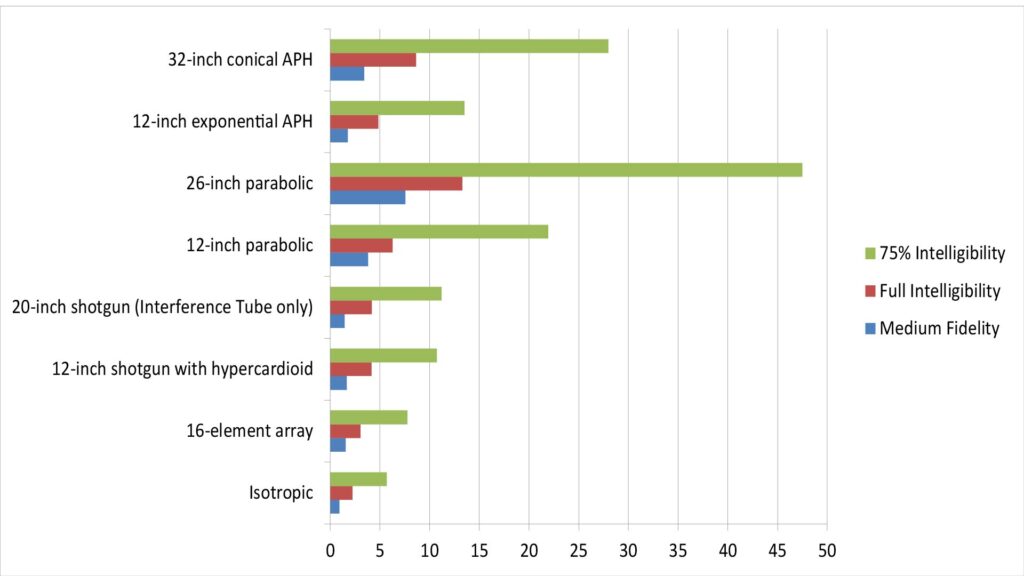
There are some obvious take-aways from this chart:
- The parabolic microphones provide the greatest range for their size, but the ranges might be much less than you’d expect. The 26-inch parabolic microphone has a range of only about 50 feet for 75-percent voice intelligibility, which is a lot less than manufacturers’ claimed ranges for such devices. However, as previously mentioned, the ranges can be quite a bit greater against louder voices.
- The 12-inch parabolic microphone easily out-ranges the 12-inch shotgun. And that’s despite the fact that the parabolic microphone isn’t augmented with a hypercardioid element to provide low-frequency directivity, as is the shotgun.
- Because of that hypercardioid behavior at low frequencies, the 12-inch shotgun has the same pick-up range as the 20-inch shotgun (which isn’t augmented with a hypercardioid).
- The 32-inch conical Acoustic Pressure Horn (APH) provides a respectable range. That range is less than that of the 26-inch parabolic, but the cheerleader’s megaphone used in the APH is a lot cheaper than a commercial 26-inch dish.
- The 12-inch exponential APH also performs surprisingly well for its size, but only if we’re interested in intelligibility and not fidelity. That’s because it has a sharp cutoff below about 700 Hz (as was evident in Figure 13).
- The 16-element array doesn’t perform much better than the reference isotropic microphone. The reason is that, while it provides 12 dB of gain, it has very little directivity over most of the audio bandwidth. However, its range advantage would be much more significant in very low ambient noise, such as in a quiet recording studio.
Final thoughts on long-range microphones
In this post I’ve described the challenges associated with picking-up sound at long ranges, summarized the various types of long-range microphones, and presented some range projections for exemplar long-range microphones. Here are the some key things I’ve learned from doing the research for this post:
- Picking-up voice at very long ranges (say 100 feet or more) isn’t possible with an unobtrusive, easily-handled device, at least under typical conditions.
- Directivity is the most important attribute in a long-range microphone, but high gain can also help.
- Predicting microphone range is trickier than it might seem, but useful predictions aren’t too hard to make.
- Each of the various types of long-range microphone have advantages and disadvantages:
- The parabolic microphone offers the greatest range for a given size, but commercial versions are pricey and they’re more fragile and harder to handle than shotgun microphones.
- Shotgun microphones are obviously quite useful, but their range advantage over conventional studio microphones is modest.
- Although much bulkier than shotgun microphone and not as effective as parabolic microphones, horn microphones might be the most cost-effective way to achieve respectable ranges.
- Small array microphones can provide significant gain, but only limited directivity…and therefore not much greater maximum range than a bare isotropic microphone element under typical conditions. However, the array’s gain can be a significant advantage in a quiet studio setting
References
- Shure website article: “Predicting speech to background noise level at the microphone,” https://service.shure.com/s/article/predicting-speech-to-background-noise-level-at-the-microphone?language=en_US [Accessed January 2022].
- Wikipedia article: “Intelligibility (communication),” https://en.wikipedia.org/wiki/Intelligibility_(communication). Accessed January 2022.
- Gerald A. Studebaker and Robert L. Sherbecoe, “Frequency-Importance and Transfer Functions for Recorded CID W-22 Word Lists ,” in Journal of Speech and Hearing Research, Volum 34, April 1991. Available at https://pubs.asha.org/doi/pdf/10.1044/jshr.3402.427; cost is $15 for non-members [accessed January 2021].